It is common to use random effects to capture heterogeneity in data that have been collected at spatial and/or temporal intervals. For example, counts of species or individuals are frequently replicated in space and time and researchers may add site or survey date as random effects in the model. These random effects are typically modeled as being normally distributed. Consider surveys \(i \in 1:I\) where counts \(y_i\) are made which we model with Poisson regression. The model with normally distributed random survey effects on the log expected count looks like this:
where the intercept \(\alpha\), the random survey-level offsets \(\epsilon_i\), and the standard deviation of the survey effects \(\tau\) are to be estimated by the model. In this post, I argue that when the random effects are not expected to be independent it almost always makes more sense to model the random effects using Gaussian processes (GPs).
GPs are a bit complicated (Simpson 2021) but one of their salient features is that any set of observations generated by a Gaussian process are marginally distributed as multivariate normal \(\textrm{Normal} (\boldsymbol{\mu}, \Sigma)\).1 In practice, the realisations of the GP are added to our linear predictor so \(\boldsymbol{\mu} = \boldsymbol{0}\). There are quite a few covariance kernels \(\Sigma\) to choose from but one of the most common is the exponentiated quadratic kernel given by \[
\Sigma_{ij} = \tau^2 \exp \left( -\frac{\lVert \boldsymbol{x}_i - \boldsymbol{x}_j \rVert^2}{2 \rho ^2} \right),
\tag{2}\]
where \(\tau^2\) is the marginal variance (analogous to variance \(\tau^2\) with normally distributed random effects), \(\rho\) is the length-scale governing the covariance between observations, and the term \(\lVert \boldsymbol{x}_i - \boldsymbol{x}_j \rVert\) is the Euclidean distance between any two points of our input.2 The length-scale \(\rho\) governs the correlation between points as a function of the distance between them. When \(\rho\) is small, there is little correlation between neighbouring locations and when \(\rho\) is large, there is high correlation between observations. Essentially, GPs allow modeling normally distributed random effects where observations close to each other (as in, surveys conducted at the same time of year) may be correlated.
Example: tadpole counts
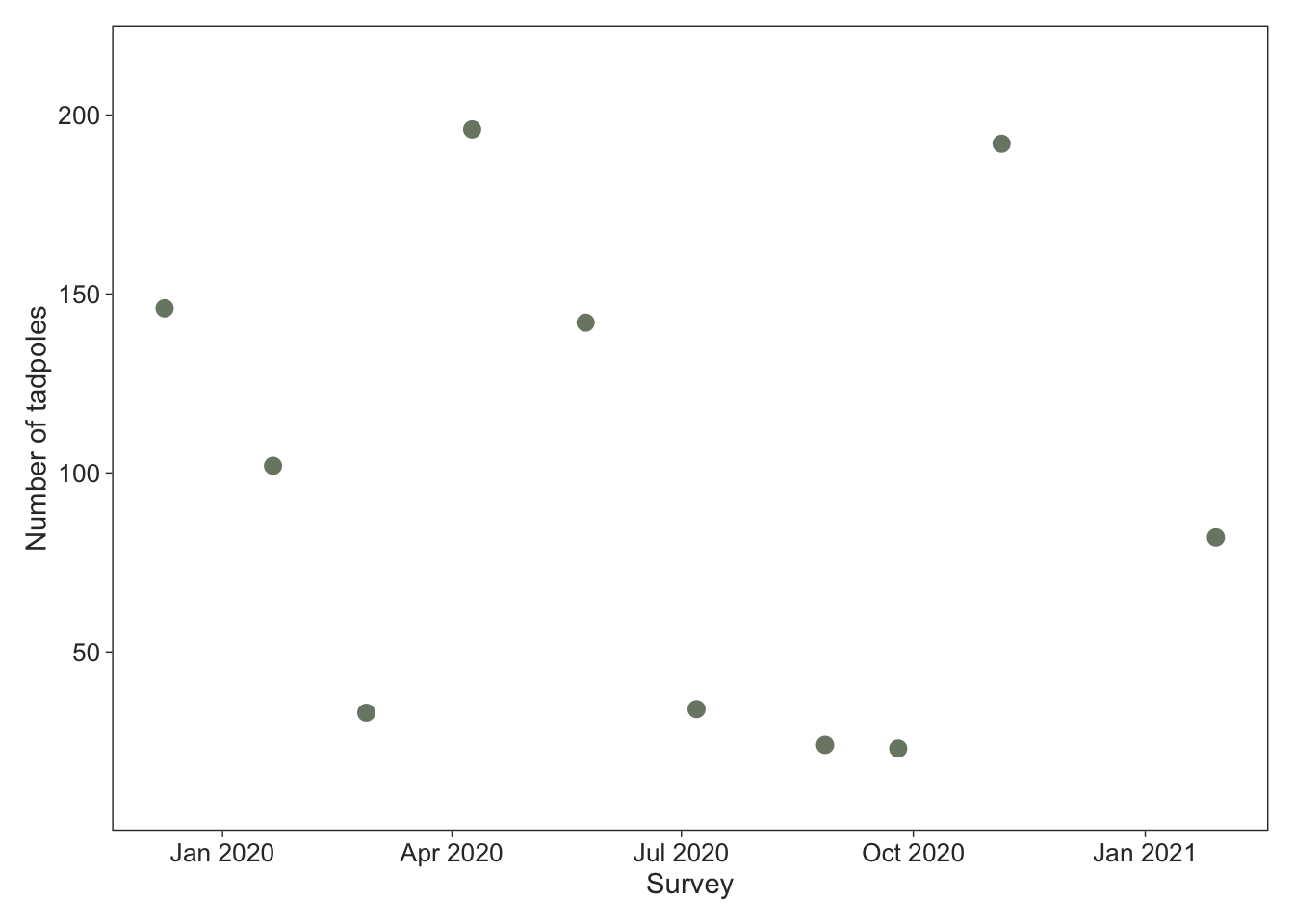
For this example, I’ll use data we collected on tadpoles of Fleay’s barred frogs (Mixophyes fleayi), a stream-dwelling species endemic to the Gondwana rainforests of northern New South Wales and southeast Queensland, Australia (Hollanders et al. 2024). During my PhD, I swept a dipnet through pools in the creeks for roughly 1 min every six weeks, deposited the tadpoles in a tub, took a photograph from above, and used Photoshop to count and measure the tadpoles.3 Here, I’ll fit the model in Equation 1 with and without GP to model the number of tadpoles I captured during each six-weekly survey at one of the sites. First I’ll download the data from my GitHub and plot the counts for the creek using ggplot2(Wickham 2016) and other packages from the tidyverse(Wickham et al. 2019).
Fleay’s barred frogs breed from the early spring to the middle of summer and generally there are several pulses of reproduction resulting in fresh cohorts of tadpoles. We’ll ignore this and just model the counts using random survey effects in the absence of any predictors.
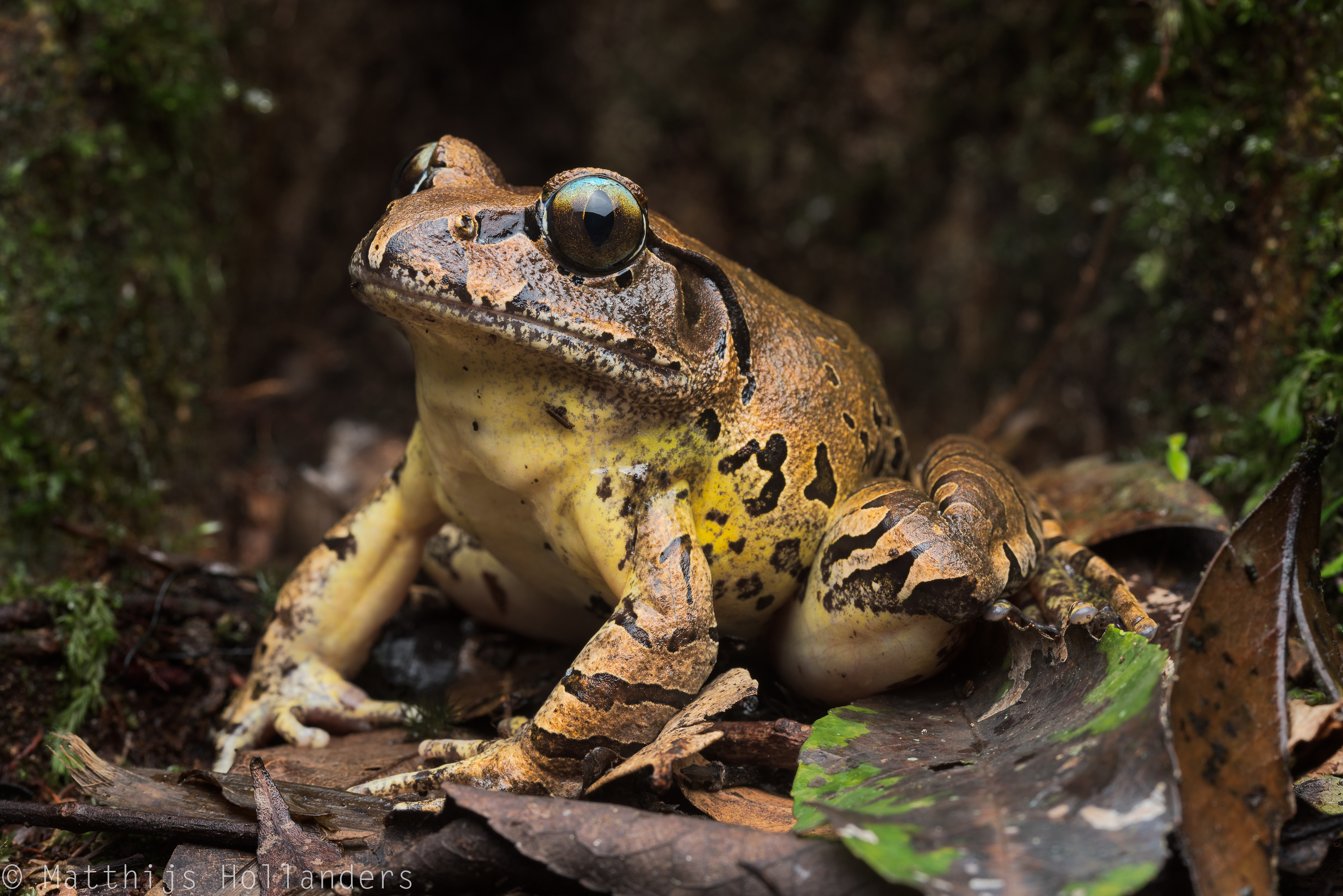
Fleay’s barred frog (Mixophyes fleayi) from Brindle Creek, Border Ranges National Park, Australia.
Setting priors for GPs
GPs have two parameters that require priors, \(\tau\) and \(\rho\). The prior for \(\tau\) can just be something like an exponential prior commonly used for standard deviations of random effects.4 The prior for the length-scale \(\rho\) is trickier as it is often not well identified by the data. In fact, the data cannot inform length-scales that are outside of the distances observed in the data. This means that we want a prior than can suppress values below and above certain thresholds. One popular distribution for length-scales that’s capable of doing exactly this is the inverse gamma distribution. Michael Betancourt’s GP case study discusses this at length and includes a function that uses Stan’s algebra solver to determine the shape and scale of the inverse gamma distribution that places a certain proportion of the probability mass between two values.5
If the study was well designed to estimate the length-scale of the GP, the survey intervals should be shorter than the minimum length-scale we think we might be dealing with. Unfortunately, I did not collect data with this question in mind, and I can easily see that the relevant length-scale is shorter than the minimum length between surveys (I surveyed at six-weekly intervals, give or take). However, for this demonstration, we’ll assume that the survey intervals were rigorously chosen and we’ll use the minimum and maximum observed temporal distances between surveys to choose a suitable inverse gamma prior for the length-scale. So, I compute the minimum and maximum distance and chose tail probabilities of 1% so that 98% of the probability mass of the length-scale falls between the minimum and maximum observed distances between the surveys.
Fitting the model
Below I write out a Stan program (Carpenter et al. 2017) that uses an indicator to use either normally distributed random effects or to use a GP with a exponentiated quadratic covariance kernel. Stan includes the handy function gp_exp_quad_cov() that generates this covariance kernel from the input (survey times expressed in weeks, in this case) and standard deviation and length-scale. We also use this GP input to pre-compute the distance matrix to get the minimum and maximum observed (temporal) distances of the surveys to use Stan’s algebra solver to determine a suitable inverse gamma prior for \(\rho\). For both types of random effects I use the non-centered parameterisation which generally has better sampling for few observations (we only have 10 data points). For GPs (and multivariate normals more generally), this entails Cholesky decomposing the covariance matrix (think of it as a matrix square root) and multiplying it by a vector of standard normal variates. Note that before Cholesky decomposing the covariance kernel, I add a diagonal matrix with a very small value (called the “nugget” or “jitter”) to ensure the matrix is positive definite.
Code
functions {// function from Michael Betancourt for inverse gamma prior shape and scalevector inv_gamma_prior(vector guess, vector theta, array[] real tails, array[] int x_i) {vector[2] params; params[1] = inv_gamma_cdf(theta[1] | guess[1], guess[2]) - tails[1]; params[2] = inv_gamma_cdf(theta[2] | guess[1], guess[2]) - tails[2];return params; }}data {int<lower=1> I; // number of surveysarray[I] real survey; // survey input as number of weeksvector[2] min_max_dist; // minimum and maximum observed distance between weeksarray[I] int y; // tadpole counts per surveyint<lower=0, upper=1> GP; // indicator for GP (0 = no, 1 = yes)}transformed data {vector<lower=0>[2] rho_prior = ones_vector(2); // length-scale prior shape and scaleif (GP) { rho_prior = algebra_solver(inv_gamma_prior, [1, 1]', min_max_dist, {0.01, 0.99}, {0});print("rho_prior: ", rho_prior); }}parameters {real alpha; // interceptreal<lower=0> tau, rho; // random effect SD and GP length-scalevector[I] z; // standard-normal z-scores for non-centered parameterisation}transformed parameters {vector[I] epsilon; // random survey effectsif (GP) { epsilon = cholesky_decompose(add_diag(gp_exp_quad_cov(survey, tau, rho), 1e-9)) * z; } else { epsilon = tau * z; }}model {// priors alpha ~ normal(0, 5); tau ~ exponential(1); rho ~ inv_gamma(rho_prior[1], rho_prior[2]); z ~ std_normal();// likelihood y ~ poisson_log(alpha + epsilon);}generated quantities {vector[I] yrep, log_lik;for (i in1:I) { yrep[i] = poisson_log_rng(alpha + epsilon[i]); log_lik[i] = poisson_log_lpmf(y[i] | alpha + epsilon[i]); }}
Running MCMC with 1 chain...

Chain 1 rho_prior: [3.58235,38.8276]
Chain 1 finished in 1.4 seconds.
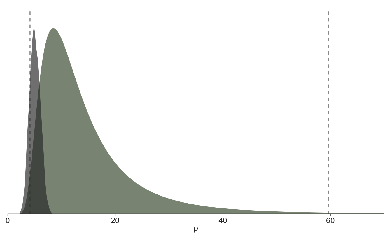
I’ll first plot the inverse gamma prior for the length-scale that was generated by the solver (green), alongside the posterior distribution of \(\rho\) (black) and the minimum and maximum observed temporal distances of the surveys (dashed lines), using the distributional(O’Hara-Wild et al. 2024) and ggdist and tidybayes packages (Kay 2024a, 2024b). The length-scale seems to want to be smaller than the prior allows, which is due to me enforcing an informative prior. Recall that I pretended the survey intervals were chosen in a principled manner to estimate this parameter by specifying a prior implying the length-scale really doesn’t be much shorter than six weeks.
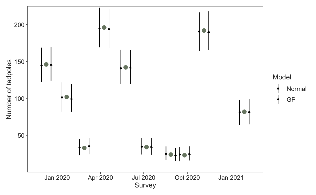
Focusing now on the posterior draws for the random survey effects \(\epsilon_i\), it’s clear that the predictions between the normal and GP model are very similar.
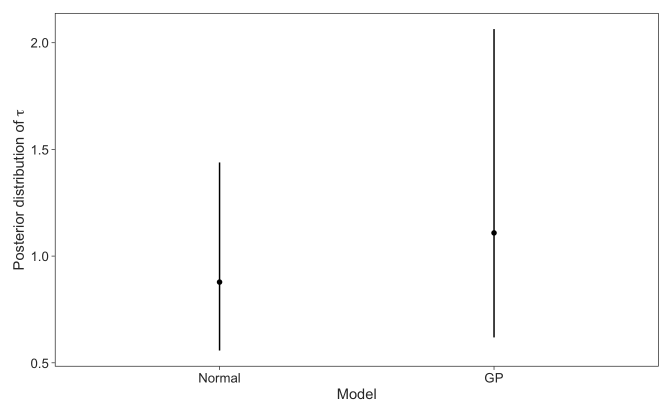
We can also see that the standard deviation of the normal model is very similar to the marginal standard deviation of the GP model, albeit with more uncertainty. To be honest, the difference in the estimates of \(\tau\) here may be driven more by our prior on \(\rho\) that may be a bit more informative than it should be.
It can be hard to interpret the parameters of the GP directly so I will make some predictions over unobserved surveys in weekly intervals. Making GP predictions involves linear algebra that I don’t pretend to fully understand. Below is some code I modified from Nicholas Clark’s excellent blog post on spatial GPs.
Code
# predicted dates and distance matrixpred_dates <-seq.Date(min(dat$date) -weeks(2), max(dat$date) +weeks(2), 7)pred <-as.numeric(pred_dates) /7dist_pred <-dist(pred) |>as.matrix()# distance matrix between observed and predicted datesdist_obs_to_pred <- proxy::dist(stan_data$survey, pred)# squared exponential kernel functiongp_exp_quad_cov <-function(dist, tau, rho, nugget =1e-9) {return(tau^2*exp(-0.5* (dist / rho)^2)) +diag(nugget, dim(dist)[1])}# function from Nicholas Clarkpredict_gp <-function(tau, rho, epsilon, dist_obs, dist_pred, dist_obs_to_pred, nugget =1e-9) {# estimated covariance kernel for the fitted points K_obs <-gp_exp_quad_cov(dist_obs, tau, rho)# estimated covariance kernel for prediction points K_pred <-gp_exp_quad_cov(dist_pred, tau, rho)# cross-covariance between fitted and prediction points K_new <-gp_exp_quad_cov(dist_obs_to_pred, tau, rho)# number of prediction points n_pred <-dim(dist_pred)[1]# posterior draw for prediction pointsreturn(t(K_new) %*%solve(K_obs, epsilon) +t(chol(K_pred -t(K_new) %*%solve(K_obs, K_new) +diag(nugget, n_pred))) %*%rnorm(n_pred))}
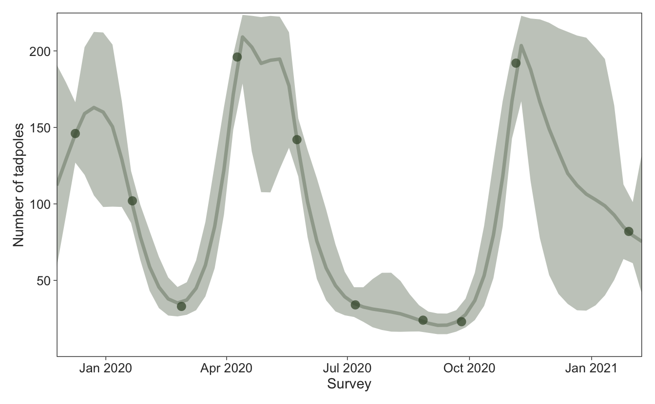
Next I extract the posterior draws of the model parameters to use the predict_gp() function for each draw to capture uncertainty. Then I plot the predictions over our existing figure. The GP was able to capture higher tadpole counts in the warmer months when reproduction is occurring, and that the winter and spring months prior to the first pulse of reproduction (July–October 2020) had low tadpole numbers. It’s possible that a different covariance kernel would work better, such as a periodic covariance kernel, but I won’t go into that here.
Using GPs to model random effects makes a lot of sense if there is some interest in modeling correlation between temporally or spatially organised data. Given that switching out the normally distributed random effects for a GP is trivial in modern probabilistic programming languages such as Stan, it makes sense to default to using them, especially as it includes involves just one extra parameter, the length-scale \(\rho\).
References
Carpenter, B., A. Gelman, M. D. Hoffman, D. Lee, B. Goodrich, M. Betancourt, M. Brubaker, J. Guo, P. Li, and A. Riddell. 2017. Stan: A Probabilistic Programming Language. Journal of Statistical Software 76:1–32.
Gabry, J., R. Češnovar, A. Johnson, and S. Bronder. 2024. cmdstanr: R Interface to “CmdStan.” manual.
Wickham, H., M. Averick, J. Bryan, W. Chang, L. D. McGowan, R. François, G. Grolemund, A. Hayes, L. Henry, J. Hester, M. Kuhn, T. L. Pedersen, E. Miller, S. M. Bache, K. Müller, J. Ooms, D. Robinson, D. P. Seidel, V. Spinu, K. Takahashi, D. Vaughan, C. Wilke, K. Woo, and H. Yutani. 2019. Welcome to the tidyverse. Journal of Open Source Software 4:1686.
Footnotes
Dan Simpson’s blog is a great place to learn more about GPs.↩︎
When our input is multidimensional, such as coordinates for spatial data, we are still working with the Euclidean distance between vectors.↩︎
I also did other things with those tadpoles, but I won’t go into that here.↩︎
This also happens to the penalised complexity (PC) prior for this parameter.↩︎
The case study is a great place to learn more about GPs more generally.↩︎