A unified approach to ecological modeling in Stan
I updated the post to replace the Viterbi algorithm (which gives the most likely sequence of latent discrete states based on the highest probabilities) with the backward sampling algorithm (which yields the most likely sequence of states by sampling them according to their probabilities) to retrieve the posterior distributions of the marginalised variables. Additionally, I made some models more efficient and updated some text and plotting.
Introduction
The development of Bayesian statistical software had considerable influence on statistical ecology because many ecological models are complex and require custom likelihoods that were not necessarily available in off-the-shelf software such as R or Program Mark (Cooch and White 2008, Kéry and Royle 2015, Kéry and Royle 2020). One of the reasons why ecological models are so complex is because the data are often messy. For instance, in something like a randomised control trial, careful design means you can make stronger assumptions such as that measurements are obtained without error. However, ecological data are noisy and we frequently require complicated observation models that account for imperfect detection of species or individuals. As a result, a large class of ecological models can be formulated as hidden Markov models (HMMs), where time-series data are modeled with a (partially or completely) unobserved ecological model and an observation model conditioned on it. Examples of ecological HMMs include mark-recapture and occupancy models, including their more complex multistate variants.
HMMs are straightforward to model with traditional Markov chain Monte Carlo (MCMC) methods because the latent ecological states can be sampled like parameters. Formulating these models became accessible to ecologists because of the simplicity afforded by statistical software like BUGS, JAGS, and NIMBLE (de Valpine et al. 2017). Consider the simple mark-recapture model where individuals \(i \in 1 : I\) first captured at time \(j = f_i\) survive between times \(j \in f_i: J\) with survival probability \(\phi\) and are recaptured on each occasion with detection probability \(p\). The state-space formulation of this model from \(j \in (f_i + 1):J\) with vague priors for \(\phi\) and \(p\) is as follows:
\[ \begin{aligned} z_{i,j} &\sim \textrm{Bernoulli} \left( z_{i,j-1} \cdot \phi \right) \\ y_{i,j} &\sim \textrm{Bernoulli} \left( z_{i,j} \cdot p \right) \\ \phi, p &\sim \textrm{Beta} \left( 1, 1 \right) \end{aligned} \tag{1}\]
where \(z_{i,j}\) are the partially observed ecological states (where \(z=1\) is an alive individual and \(z=0\) is a dead individual) and \(y_{i,j}\) are the observed data (where \(y=1\) is an observed individual and \(y=0\) is an unobserved individual). Using NIMBLE 1.1.0 in R 4.3.2 (R Core Team 2023), coding this model is straightforward and follows the algebra above closely.
After simulating some data, creating a NIMBLE model from the code, and configuring the MCMC, we can see that each unknown z[i, j] gets its own binary MCMC sampler.
Code
# metadata and parameters
I <- 100
J <- 8
phi <- 0.6
p <- 0.7

# containers
z <- y <- z_known <- matrix(NA, I, J)
f <- sample(1:(J - 1), I, replace = T) |> sort()
l <- numeric(I)

# simulation
for (i in 1:I) {
  z[i, f[i]] <- y[i, f[i]] <- 1
  for (j in (f[i] + 1):J) {
    z[i, j] <- rbinom(1, 1, z[i, j - 1] * phi)
    y[i, j] <- rbinom(1, 1, z[i, j] * p)
  } # t
  l[i] <- max(which(y[i, ] == 1))
  z_known[i, f[i]:l[i]] <- 1
} # i

# create NIMBLE model object
Rmodel <- nimbleModel(cmr_code,
                      constants = list(I = I, J = J, f = f),
                      data = list(y = y, z = z_known))

# configure MCMC
conf <- configureMCMC(Rmodel)
===== Monitors =====
thin = 1: p, phi
===== Samplers =====
RW sampler (2)
- phi
- p
binary sampler (372)
- z[] (372 elements)Note that because we know with certainty that individuals were alive between the first and last survey they were captured, we can actually ease computation by supplying those z[i, f[i]:l[i]] as known. We’ll run this model to confirm that it’s able to recover our input parameters using MCMCvis (Youngflesh 2018).
Code
# A tibble: 2 × 9
  variable  mean     sd `2.5%` `50%` `97.5%`  Rhat n.eff truth
  <chr>    <dbl>  <dbl>  <dbl> <dbl>   <dbl> <dbl> <dbl> <dbl>
1 phi      0.532 0.0415  0.452 0.530   0.621  1.02   549   0.6
2 p        0.711 0.0672  0.579 0.711   0.839  1.01   319   0.7
As flexible as Bayesian software like BUGS and JAGS are, most of them do not use Hamiltonian Monte Carlo (HMC, Neal 1994) to generate samples from the posterior distribution (but see nimbleHMC for a recent implementation in NIMBLE). Without going into detail myself1, HMC is considered a superior algorithm and moreover gives warnings when something goes wrong in the sampling, alerting the user to potential issues in estimation. As a result, HMC should generally be preferred by practitioners but it has one trait that can be challenging to ecologists in particular: it requires that all parameters are continuous, meaning that our typical state-space formulations of HMMs cannot be fit with HMC due to the presence of discrete parameters like our ecological states z[i, j] above. The remainder of this post will focus on dealing with fitting complex ecological models using Stan (Carpenter et al. 2017), a probabilistic programming language which implements a state-of-the-art No U-Turn Sampler (NUTS, Hoffman and Gelman 2014). I present a unified approach that is applicable to simple and complex models alike, highlighted with three examples of increasing complexity.
Marginalisation
Since HMC cannot sample discrete parameters, we have to reformulate our models without the latent states through a process called marginalisation. Marginalisation essentially just counts the mutually exclusive ways an observation can be made and sums these probabilities, as \(\Pr(A \cup B) = \Pr(A) + \Pr(B)\). For instance, in the above mark-recapture example, consider an individual was captured on occasion 1 and recaptured on occasion 2. The only way this could have happened is that the individual survived the interval with probability \(\phi\) and was recaptured on occasion 2 with probability \(p\), making the marginal likelihood of that datapoint \(\phi \cdot p\). However, if it was not observed at time 2, two things are possible: either the animal survived but was not recaptured with probability \(\phi \cdot (1 - p)\) or the individual died with probability \(1 - \phi\) and was thus not recaptured. Summing these probabilities gives us the marginal likelihood for that datapoint, which is \(\phi \cdot (1 - p) + (1 - \phi)\). Models can be marginalised in many different ways, but in this post I’m going to focus on the forward algorithm. Although it takes some getting used to, the forward algorithm facilitates fitting a wide variety of (increasingly complex) HMMs.
Forward algorithm
First, I’m going to restructure our mark-recapture model as a multistate model with the introduction of transition probability matrices (TPMs), which I denote as \(P\) in the equations. In the mark-recapture example, we still have two latent ecological states, (1) alive and (2) dead. The transitions from one state to the other is given by the following TPM, where the states of departure (survey \(j - 1\)) are in the rows and states of arrival (survey \(j\)) are in the columns (note that the rows of a row-stochastic TPM must sum to 1):
\[ P_z = \begin{bmatrix} \phi & 1 - \phi \\ 0 & 1 \end{bmatrix} \tag{2}\]
Here, the dead state is an absorbing state and individuals remain in the alive states with probability \(\phi\). The observation process still deals with two observed states, (1) not detected and (2) detected, and is also formulated as a \(2 \cdot 2\) TPM, where the ecological states are in the rows (states of departure) and the observed states in the columns (states of arrival):
\[ P_y = \begin{bmatrix} 1 - p & p \\ 1 & 0 \end{bmatrix} \tag{3}\]
The forward algorithm works by computing the marginal likelihood of an individual being in each state \(s \in 1 : S\) at survey \(j\) given the observations up to \(j\), stored in a \(S \cdot J\) matrix we’ll call \(\Omega\). From here on, the notation for subsetting row \(i\) of a matrix \(M\) is \(M_i\) and \(M_{:j}\) for subsetting column \(j\). The forward algorithm starts from a vector of initial state probabilities, which in the mark-recapture example are known, given that we know with certainty that every individual is alive at first capture:
\[ \Omega_{:{f_i}} = \left[ 1, 0 \right]^\intercal \tag{4}\]
For subsequent occasions after an individual’s first capture \(j \in (f_i+1):J\), the marginal probabilities of being in state \(s\) at time \(j\) are computed as:
\[ \Omega_{:j} = P_z^\intercal \cdot \Omega_{:j-1} \odot {P_y}_{[:y_{i, j}]} \tag{5}\]
That is, matrix multiplying the transposed ecological TPM wih the vector of marginal probabilities at time \(j-1\) and then element-wise multiplying (where \(\odot\) denotes the Hadamard or element-wise product) the resulting vector with the relevant column of the observation TPM, where the first column is used if the individual was not observed (\(y_{i,j} = 1\)) and the second column if it was observed (\(y_{i,j} = 2\)). This process continues iteratively until survey \(J\) after which the log density is incremented with the log of the sum of \(\Omega_{:J}\), the marginal probabilities of being in each state at the end of the study period.
Posterior distributions for the discrete parameters
After marginalising the discrete variables from the model, we are frequently still interested in estimates for these quantities. For instance, in mark-recapture models we often want to estimate population sizes or in occupancy models we want to know the proportion of our sampled sites that were occupied. Ironically, we can actually get better estimates of the posterior distribution of the discrete variables after marginalising because of better exploration of the tails.2. In order to do so, we use the backward algorithm to generate a posterior distribution over the most likely state sequence. We start by sampling the most likely final state \(z_{i,J}\) by sampling from the associated probabilities, which we can do in Stan using the categorical_rng() function after normalising them (dividing by the sum of the probabilities). Then we work backwards to compute the most likely state that came prior, by sampling from the probabilities given by the marginal probabilities of each state at time \(J-1\) and having transitioned to state \(z_{i,J}\), \(\Omega_{:J-1} \odot {P_z}_{[:z_{i,J}]}\). We do this recursively until \(j=1\) (or in case of mark-recapture, until the survey after the last capture, as we know the individual was alive until then).
Example 1: Basic mark-recapture as a HMM
As a first example of structuring ecological models as HMMs using the forward algorithm, I have translated the initial mark-recapture model for use in Stan. Stan programs specify a log density, so I wrote two versions, one with the probabilities which most closely resembles the above algebra and one using log probabilities throughout. Doing so involves swapping the multiplication of probabilities with summing the log probabilities, changing log(sum()) to log_sum_exp(), and performing matrix multiplication on the log scale with a custom function log_prod_exp()3, which I found on Stack Overflow (note that the function is overloaded to account for the dimensions of your two matrices). I have a few comments:
- Just like in the NIMBLE version, we don’t have to worry about the probabilities associated with being dead between the first and last capture. Note that for the occasions between first and last capture, I only compute the marginal probabilities of the alive state. At the occasion of last capture, I fix \(\Omega_{3,l_i}\) to 0 (or
negative_infinity()for log). - In all models, I also compute the site-level log likelihood in the vector
log_likfor potential use in model checking using the loo package (Vehtari et al. 2023). - Most parts of the
modelblock are repeated ingenerated quantities. Although this makes the whole program more verbose, it is more efficient to compute derived quantities in thegenerated quantitiesblock as they are only computed once per HMC iteration, whereas thetransformed parametersand themodelblocks get updated with each gradient evaluation, of which there can be many per iteration.
Stan programs
Code
functions {
  // normalise a vector of probabilities
  vector normalise(vector A) {
    return A / sum(A);
  }
}

data {
  int<lower=1> I, J;
  array[I] int<lower=1, upper=J> f;
  array[I] int<lower=f, upper=J> l;
  array[I, J] int<lower=1, upper=2> y;
}

parameters {
  real<lower=0, upper=1> phi, p;
}

model {
  // priors
  target += beta_lupdf(phi | 1, 1);
  target += beta_lupdf(p | 1, 1);

  // TPMs
  matrix[2, 2] P_z, P_y;
  P_z = [[ phi, 1 - phi ],
         [ 0, 1 ]];
  P_y = [[ 1 - p, p ],
         [ 1, 0 ]];

  // forward algorithm
  matrix[2, J] Omega;
  for (i in 1:I) {

    // initial state probabilities
    Omega[:, f[i]] = [ 1, 0 ]';

    // must be alive up until last capture
    for (j in (f[i] + 1):l[i]) {
      Omega[1, j] = P_z[1, 1] * Omega[1, j - 1] * P_y[1, y[i, j]];
    }
    Omega[2, l[i]] = 0;

    // after last capture, condition both states on being undetected
    for (j in (l[i] + 1):J) {
      Omega[:, j] = P_z' * Omega[:, j - 1] .* P_y[:, 1];
    }

    // increment log density
    target += log(sum(Omega[:, J]));
  }
}

generated quantities {
  vector[I] log_lik;
  array[I, J] int z;
  {
    matrix[2, 2] P_z, P_y;
    P_z = [[ phi, 1 - phi ],
           [ 0, 1 ]];
    P_y = [[ 1 - p, p ],
           [ 1, 0 ]];
    matrix[2, J] Omega;
    for (i in 1:I) {

      // forward algorithm for log likelihood
      Omega[:, f[i]] = [ 1, 0 ]';
      for (j in (f[i] + 1):l[i]) {
        Omega[1, j] = P_z[1, 1] * Omega[1, j - 1] * P_y[1, y[i, j]];
      }
      Omega[2, l[i]] = 0;
      for (j in (l[i] + 1):J) {
        Omega[:, j] = P_z' * Omega[:, j - 1] .* P_y[:, 1];
      }
      log_lik[i] = log(sum(Omega[:, J]));

      // backward algorithm for ecological states
      z[i, J] = categorical_rng(normalise(Omega[:, J]));
      for (j in (l[i] + 1):(J - 1)) {
        int jj = J + l[i] - j;  // reverse indexing
        z[i, jj] = categorical_rng(normalise(Omega[:, jj]
                                             .* P_z[:, z[i, jj + 1]]));
      }
      // alive from first to last capture
      z[i, f[i]:l[i]] = ones_int_array(l[i] - f[i] + 1);
    }
  }
}
Code
functions{
  // normalise a vector of log probabilities
  vector normalise_log(vector A) {
    return A - log_sum_exp(A);
  }

  /**
   * Return the natural logarithm of the product of the element-wise
   * exponentiation of the specified matrices
   *
   * @param A  First matrix or (row_)vector
   * @param B  Second matrix or (row_)vector
   *
   * @return   log(exp(A) * exp(B))
   */
  matrix log_prod_exp(matrix A, matrix B) {
    int I = rows(A);
    int J = cols(A);
    int K = cols(B);
    matrix[J, I] A_tr = A';
    matrix[I, K] C;
    for (k in 1:K) {
      for (i in 1:I) {
        C[i, k] = log_sum_exp(A_tr[:, i] + B[:, k]);
      }
    }
    return C;
  }
  vector log_prod_exp(matrix A, vector B) {
    int I = rows(A);
    int J = cols(A);
    matrix[J, I] A_tr = A';
    vector[I] C;
    for (i in 1:I) {
      C[i] = log_sum_exp(A_tr[:, i] + B);
    }
    return C;
  }
  row_vector log_prod_exp(row_vector A, matrix B) {
    int K = cols(B);
    vector[size(A)] A_tr = A';
    row_vector[K] C;
    for (k in 1:K) {
      C[k] = log_sum_exp(A_tr + B[:, k]);
    }
    return C;
  }
  real log_prod_exp(row_vector A, vector B) {
    return log_sum_exp(A' + B);
  }
}

data {
  int<lower=1> I, J;
  array[I] int<lower=1, upper=J - 1> f;
  array[I] int<lower=f, upper=J> l;
  array[I, J] int<lower=1, upper=2> y;
}

parameters {
  real<lower=0, upper=1> phi, p;
}

model {
  // priors
  target += beta_lupdf(phi | 1, 1);
  target += beta_lupdf(p | 1, 1);

  // (log) TPMs
  matrix[2, 2] P_z, P_y;
  P_z = [[ phi, 1 - phi ],
         [ 0, 1 ]];
  P_y = [[ 1 - p, p ],
         [ 1, 0 ]];
  P_z = log(P_z);
  P_y = log(P_y);

  // forward algorithm
  matrix[2, J] Omega;
  for (i in 1:I) {

    // initial state log probabilities
    Omega[:, f[i]] = [ 0, negative_infinity() ]';

    // must be alive up until last capture
    for (j in (f[i] + 1):l[i]) {
      Omega[1, j] = P_z[1, 1] + Omega[1, j - 1] + P_y[1, y[i, j]];
    }
    Omega[2, l[i]] = negative_infinity();

    // after last capture, condition both states on being undetected
    for (j in (l[i] + 1):J) {
      Omega[:, j] = log_prod_exp(P_z', Omega[:, j - 1]) + P_y[:, 1];
    }

    // increment log density
    target += log_sum_exp(Omega[:, J]);
  }
}

generated quantities {
  array[I, J] int z;
  vector[I] log_lik;
  {
    matrix[2, 2] P_z, P_y;
    P_z = [[ phi, 1 - phi ],
           [ 0, 1 ]];
    P_y = [[ 1 - p, p ],
           [ 1, 0 ]];
    P_z = log(P_z);
    P_y = log(P_y);
    matrix[2, J] Omega;
    for (i in 1:I) {

      // forward algorithm for log likelihood
      Omega[:, f[i]] = [ 0, negative_infinity() ]';
      for (j in (f[i] + 1):l[i]) {
        Omega[1, j] = P_z[1, 1] + Omega[1, j - 1] + P_y[1, y[i, j]];
      }
      Omega[2, l[i]] = negative_infinity();
      for (j in (l[i] + 1):J) {
        Omega[:, j] = log_prod_exp(P_z', Omega[:, j - 1]) + P_y[:, 1];
      }
      log_lik[i] = log_sum_exp(Omega[:, J]);

      // backward algorithm for ecological states
      z[i, J] = categorical_rng(exp(normalise_log(Omega[:, J])));
      for (j in (l[i] + 1):(J - 1)) {
        int jj = J + l[i] - j;  // reverse indexing
        z[i, jj] = categorical_rng(exp(normalise_log(Omega[:, jj]
                                                     + P_z[:, z[i, jj + 1]])));
      }
      // alive from first to last capture
      z[i, f[i]:l[i]] = ones_int_array(l[i] - f[i] + 1);
    }
  }
}
Why we like HMC
Using CmdStanR 0.7.1 to call CmdStan 2.34.1 (Gabry et al. 2023), we’ll just run the log probability model for the same number of iterations as the NIMBLE version, and we see that there were no issues with sampling (Stan would tell us otherwise) and the effective sample sizes (ESS) were several times higher than for the NIMBLE model.
Code
# data for Stan without NAs
cmr_data <- list(I = I, J = J, f = f, l = l, y = y + 1) |>
  sapply(\(x) replace(x, is.na(x), 1))

# run HMC
library(cmdstanr)
options(mc.cores = n_chains)
fit_cmr <- cmr_lp$sample(data = cmr_data, refresh = 0, chains = n_chains,
                         iter_warmup = n_iter, iter_sampling = n_iter)
Running MCMC with 8 parallel chains...
Chain 1 finished in 1.4 seconds.
Chain 4 finished in 1.4 seconds.
Chain 6 finished in 1.3 seconds.
Chain 2 finished in 1.4 seconds.
Chain 3 finished in 1.5 seconds.
Chain 5 finished in 1.4 seconds.
Chain 7 finished in 1.3 seconds.
Chain 8 finished in 1.4 seconds.
All 8 chains finished successfully.
Mean chain execution time: 1.4 seconds.
Total execution time: 1.5 seconds.Code
# A tibble: 2 × 8
  variable median    q5   q95 ess_bulk ess_tail ess_nimble truth
  <chr>     <dbl> <dbl> <dbl>    <dbl>    <dbl>      <dbl> <dbl>
1 phi       0.529 0.459 0.596    2127.    2315.        549   0.6
2 p         0.719 0.599 0.819    2084.    2219.        319   0.7
Computed from 4000 by 100 log-likelihood matrix.

         Estimate   SE
elpd_loo   -151.1 14.8
p_loo         2.2  0.7
looic       302.2 29.7
------
MCSE of elpd_loo is 0.0.
MCSE and ESS estimates assume MCMC draws (r_eff in [0.4, 1.0]).

All Pareto k estimates are good (k < 0.7).
See help('pareto-k-diagnostic') for details.
And just to confirm, we check if the backward algorithm was able to closely recover the latent alive states. In order to assess this fairly, I’ll only check what proportion of the ambiguous states (i.e., after last capture) was estimated correctly, based on the posterior medians.
Example 2: Dynamic multistate occupancy model
In order to highlight the generality of the above modeling approach, we’re going to switch gears to a dynamic occupancy model. There are some trivial to implement differences with the basic mark-recapture model that can seem daunting at first:
- There can be more than two states.
- The initial state probabilities here are unknown, that is, we don’t know the occupancy state of a site when it’s first surveyed.
- State transitions can happen in more than one direction, whereas dead individuals in mark-recapture can never transition to alive (i.e., there is no absorbing state).
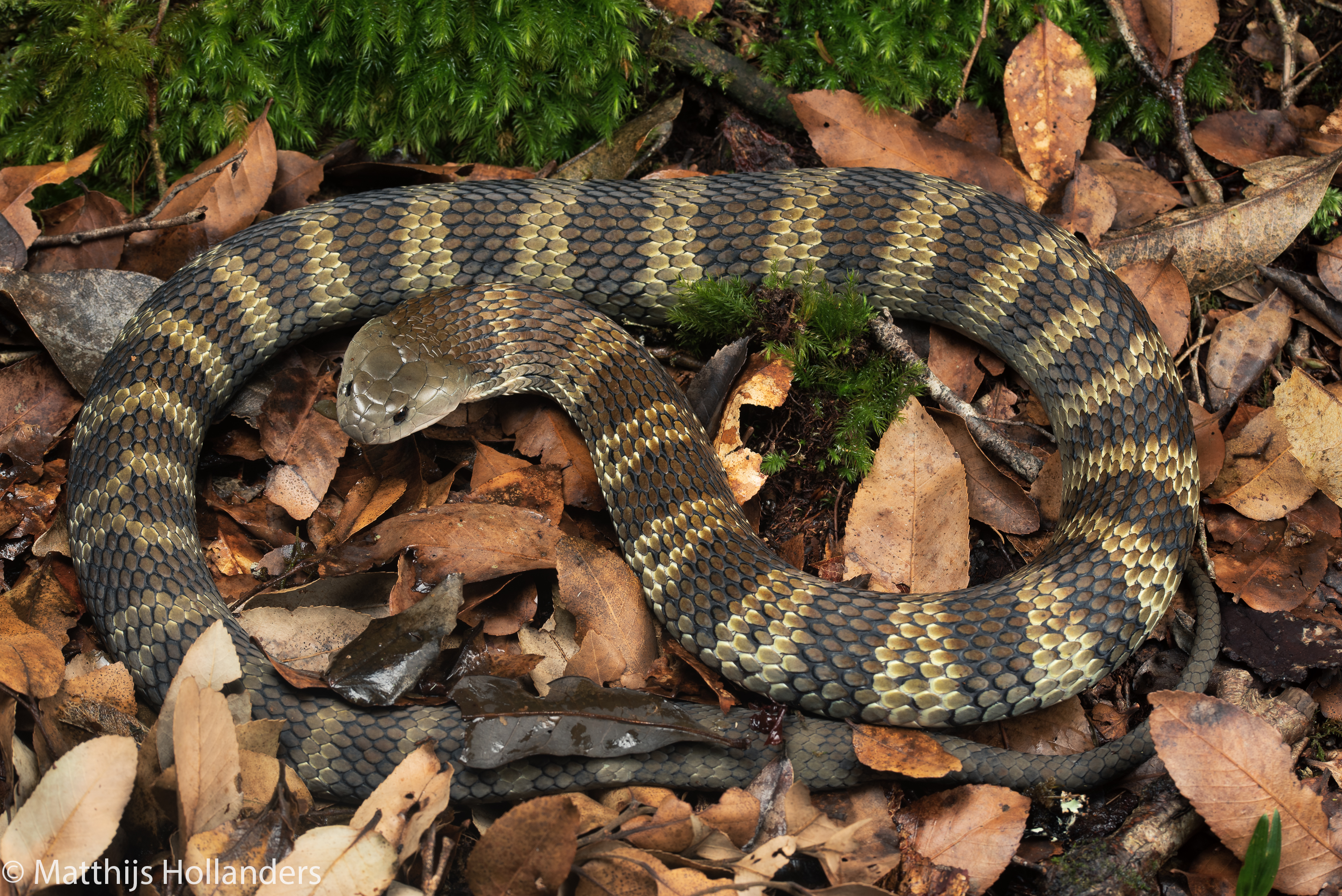
Consider a study area containing sites \(i \in 1 : I\) surveyed across seasons \(j \in 1 : J\). We are investigating whether sites are occupied by tiger snakes (Notechis scutatus) in each season, but want to differentiate between sites that simply support tiger snakes or those that support breeding. Our ecological process thus has three possible states: (1) unoccupied by tiger snakes, (2) occupied by tiger snakes but not for breeding, or (3) occupied by breeding tiger snakes. The observation process also has three possible states: (1) no snakes found, (2) snakes found but no evidence of breeding, and (3) snakes found with evidence of breeding, as determined by the discovery of gravid females. Instead of directly formulating the ecological TPM here, we’ll do it in continuous time instead using a transition rate matrix (TRM), which I call \(Q\) in the equations. Although this may not be the best example for use with a continuous time model, I think it comes up often enough in these ecological models to warrant a demonstration.
TPMs assume equal intervals between surveys, but this is the exception rather than the norm for ecological data. Although things like survival probabilities can easily be exponentiated to the time interval, this doesn’t work for processes that are not absorbing states, i.e., snakes moving in and out of sites. Unlike individual survival, sites are free to transition between states from year to year. Even with simpler models, however, it often makes more sense to model the survival process with mortality hazard rates (where the survival probability \(S\) is related to the mortality hazard rate \(h\) as \(S = \exp(-h)\)) for a number of reasons (Ergon et al. 2018). The multistate extension of this is straightforward, where we instead take the matrix exponential of a TRM (Glennie et al. 2022). By constructing our transition matrices as TRMs, where the off-diagonals contain instantaneous hazard rates and the diagonals contain negative sums of these off-diagonals (ensuring rows sum to 0, not 1), we can generate time-specific TPMs by taking the matrix exponential of the TRM multiplied by the time interval between occasions (\(\tau_j\)), thereby essentially marginalising over possible state transitions that occurred during survey intervals:
\[ {P_z}_{[j]} = \exp \left( Q \cdot \tau_j \right) \tag{6}\]
A TRM for the tiger snake example might look something like this, with again states of departure (season \(j-1\)) in the rows and states of arrival (season \(j\)) in the columns:
\[ Q = \begin{bmatrix} -(\gamma_1 + \gamma_2) & \gamma_1 & \gamma_2 \\ \epsilon_1 & -(\epsilon_1 + \psi_1) & \psi_1 \\ \epsilon_2 & \psi_2 & -(\epsilon_2 + \psi_2) \end{bmatrix} \tag{7}\] with the following parameters:
- \(\gamma_1\): the “non-breeding” colonisation rate, or the rate at which a site becomes occupied with non-breeding snakes at time \(j\) when the site was not occupied at time \(j - 1\).
- \(\gamma_2\): the “breeding” colonisation rate, or the rate at which a site becomes occupied with breeding snakes at time \(j\) when the site was not occupied at time \(j - 1\).
- \(\epsilon_1\): the “non-breeding” emigration rate, or the rate at which a site becomes onoccupied at time \(j\) when it was occupied with non-breeding snakes at time \(j - 1\).
- \(\epsilon_2\): the “breeding” emigration rate, or the rate at which a site becomes onoccupied at time \(j\) when it was occupied with breeding snakes at time \(j - 1\).
- \(\psi_1\): the breeding rate, or the rate at which a site becomes used for breeding at time \(j\) when the site was occupied but not used for breeding at time \(j - 1\).
- \(\psi_2\): the breeding cessation rate, or the rate at which a site stops being used for breeding at time \(j\) when the site was used for breeding at time \(j - 1\).
Note that even if these parameters aren’t exactly the quantities of interest, derivations of these parameters are easily produced as generated quantities after parameter estimation. Of course, these parameters can be modeled more complexly with linear or non-linear effects at the level of years, sites, or both, with the only changes being that the TRMs are constructed at those levels (for instance, by creating site- and year-level TRMs where the parameters populating the TRM are allowed to vary at that level—see Example 3 for an application).
In addition to the TRM/TPM, the ecological process is initiated on the first occasion with an initial state vector, giving the probabilities of being in each state at \(j = 1\):
\[ \boldsymbol{\eta} = \left[ \eta_1 , \eta_2 , \eta_3 \right] \tag{8}\]
Simulating continuous time
Below, I’ll simulate the ecological data by specifying a TRM and using the expm package to take the matrix exponential to generate the TPMs (Goulet et al. 2021). In order to simulate ecological states z[i, j] we use the categorical distribution, which is just the Bernoulli distribution generalised to multiple outcomes. I demonstrate the ability to accommodate unequal time intervals with the TRM.
Code
# metadata
I <- 100
J <- 10
K_max <- 4
tau <- rlnorm(J - 1)

# parameters
eta <- c(NA, 0.3, 0.4)       # unoccupied/non-breeding/breeding initial probabilities
eta[1] <- 1 - sum(eta[2:3])  # ensure probabilities sum to 1 (simplex)
gamma <- c(0.3, 0.2)         # non-breeding/breeding colonisation rates
epsilon <- c(0.4, 0.1)       # non-breeding/breeding emigration rates
psi <- c(0.4, 0.3)           # breeding/breeding cessation rates

# function for random categorical draw
rcat <- function(n, prob) {
  return(
    rmultinom(n, size = 1, prob) |>
      apply(2, \(x) which(x == 1))
  )
}

# TRM
Q <- matrix(c(-(gamma[1] + gamma[2]), gamma[1], gamma[2],
              epsilon[1], -(epsilon[1] + psi[1]), psi[1],
              epsilon[2], psi[2], -(epsilon[2] + psi[2])),
            3, byrow = T)
Q
[,1] [,2] [,3]
[1,] -0.5 0.3 0.2
[2,] 0.4 -0.8 0.4
[3,] 0.1 0.3 -0.4Code
       [,1]  [,2]   [,3]
[1,] 0.9036 0.056 0.0404
[2,] 0.0739 0.851 0.0754
[3,] 0.0214 0.056 0.9226
Code
      [,1] [,2] [,3] [,4] [,5] [,6] [,7] [,8] [,9] [,10]
 [1,]    1    1    1    2    1    1    1    2    2     3
 [2,]    2    2    3    3    1    1    3    2    1     1
 [3,]    1    1    2    3    2    2    3    1    1     2
 [4,]    3    3    2    3    1    1    3    3    3     3
 [5,]    3    3    3    3    2    1    1    1    1     3
 [6,]    1    1    3    2    3    2    1    1    1     1
 [7,]    3    3    2    2    1    2    3    3    2     3
 [8,]    3    3    3    3    3    2    2    2    2     2
 [9,]    1    1    2    2    3    3    3    1    3     3
[10,]    3    3    3    3    2    2    2    3    3     1
Observation process
Although possible to construct in continuous time, often our observation model makes more sense in discrete time, especially if specific surveys were conducted instead of with something like an automated recording device. For instance, with dynamic occupancy models, an investigator would conduct multiple “secondary” surveys \(k \in 1:K_{ij}\) within a season in order to disentangle the ecological process from the observation process.
With multistate models where individuals or sites can transition between ecological states, in order to reliably estimate transitions rates and detection probabilities we need to conduct multiple consecutive surveys within periods of assumed closure, yielding secondary surveys nested within primary occasions. In the absence of this, there are parameter identifiability issues for the state transition rates and state-specific detection probabilities. This survey strategy was originally called the “robust design” (Pollock 1982) and the necessity of applying it for multistate models more generally has gone largely unappreciated by ecologists.
As in the mark-recapture example, we construct an observation TPM where the ecological states are in the rows and observed states in the columns, recognising that there’s uncertainty in being able to detect breeding:
\[ P_y = \begin{bmatrix} 1 & 0 & 0 \\ 1 - p_1 & p_1 & 0 \\ 1 - p_2 & p_2 \cdot (1 - \delta) & p_2 \cdot \delta \end{bmatrix} \tag{9}\] with the following parameters:
- \(p_{1:2}\): the state-specific detection probabilities, or the probabilities of detecting tiger snakes if they are present but not breeding (\(p_1\)) or present and breeding (\(p_2\)).
- \(\delta\): the breeding detection probability, or the probability of detecting tiger snake breeding conditional on it occurring at a site. Note that in this example, breeding is detected when gravid females are found. Note that false-positive detections of any kind (erroneous snake identification, etc.) are not considered, but will be in Example 3.
I’ll simulate some observational data below where the investigators aimed to conduct 4 secondary surveys per site and primary occasion (\(K_{i,j}\)), all conducted during the tiger snake breeding season, with some secondary surveys missed, and some years missed altogether (simulated as \(K_{i,j} = 0\)).
Code
# parameters
p <- c(0.4, 0.5)  # non-breeding/breeding detection probabilities
delta <- 0.6      # breeding detection probability

# TPM
P_y <- matrix(c(1, 0, 0,
                1 - p[1], p[1], 0,
                1 - p[2], p[2] * (1 - delta), p[2] * delta),
              3, byrow = T)

# containers
K <- matrix(sample(0:K_max, I * J, replace = T), I, J)
y <- array(NA, c(I, J, K_max))

# simulation
for (i in 1:I) {
  for (j in 1:J) {
    if (K[i, j]) {
      y[i, j, 1:K[i, j]] <- rcat(K[i, j], P_y[z[i, j], ])
    }
  }
}
Stan program
Below is the Stan program for the above model written with log probabilities. In many ways it is similar to the mark-recapture example, with the following noteworthy changes:
- When no surveys were done in a season (
K[i, j] = 0), Stan will automatically skip over them because a loopfor (k in 1:0)is ignored, unlike in R! - All entries in the \(3 \cdot J\) matrix
Omegaare initialised with the observation process. For each secondary survey, I subset the appropriate column from \(P_y\) and increment it onto \(\Omega_{:,j}\). The marginal likelihood of the observation process is just the sum of the respective log probabilities. - The continuous time transition rates \(\gamma\), \(\epsilon\), and \(\psi\) are given Exponential(3) priors, as these are good priors when the snapshot property of HMMs is satisfied (see Equation 2 in (Goulet et al. 2021)).
Code
functions{
  // normalise a vector of log probabilities
  vector normalise_log(vector A) {
    return A - log_sum_exp(A);
  }

  /**
   * Return the natural logarithm of the product of the element-wise
   * exponentiation of the specified matrices
   *
   * @param A  First matrix or (row_)vector
   * @param B  Second matrix or (row_)vector
   *
   * @return   log(exp(A) * exp(B))
   */
  matrix log_prod_exp(matrix A, matrix B) {
    int I = rows(A);
    int J = cols(A);
    int K = cols(B);
    matrix[J, I] A_tr = A';
    matrix[I, K] C;
    for (k in 1:K) {
      for (i in 1:I) {
        C[i, k] = log_sum_exp(A_tr[:, i] + B[:, k]);
      }
    }
    return C;
  }
  vector log_prod_exp(matrix A, vector B) {
    int I = rows(A);
    int J = cols(A);
    matrix[J, I] A_tr = A';
    vector[I] C;
    for (i in 1:I) {
      C[i] = log_sum_exp(A_tr[:, i] + B);
    }
    return C;
  }
  row_vector log_prod_exp(row_vector A, matrix B) {
    int K = cols(B);
    vector[size(A)] A_tr = A';
    row_vector[K] C;
    for (k in 1:K) {
      C[k] = log_sum_exp(A_tr + B[:, k]);
    }
    return C;
  }
  real log_prod_exp(row_vector A, vector B) {
    return log_sum_exp(A' + B);
  }
}

data {
  int<lower=1> I, J, K_max;
  array[I, J] int<lower=0, upper=K_max> K;
  vector<lower=0>[J - 1] tau;
  array[I, J, K_max] int<lower=1, upper=3> y;
}

parameters {
  simplex[3] eta;
  vector<lower=0>[2] gamma, epsilon, psi;
  vector<lower=0, upper=1>[2] p;
  real<lower=0, upper=1> delta;
}

model {
  // priors
  target += dirichlet_lupdf(eta | ones_vector(3));
  target += exponential_lupdf(gamma | 3);
  target += exponential_lupdf(epsilon | 3);
  target += exponential_lupdf(psi | 3);
  target += beta_lupdf(p | 1, 1);
  target += beta_lupdf(delta | 1, 1);

  // log initial state probabilities, TRM, and log TPMs
  vector[3] log_eta = log(eta);
  matrix[3, 3] Q, P_y;
  array[J - 1] matrix[3, 3] P_z;
  Q = [[ -(gamma[1] + gamma[2]), gamma[1], gamma[2] ],
       [ epsilon[1], -(epsilon[1] + psi[1]), psi[1] ],
       [ epsilon[2], psi[2], -(epsilon[2] + psi[2]) ]];
  for (j in 2:J) {
    P_z[j - 1] = matrix_exp(Q * tau[j - 1]);
  }
  P_z = log(P_z);
  P_y = [[ 1, 0, 0 ],
         [ 1 - p[1], p[1], 0 ],
         [ 1 - p[2], p[2] * (1 - delta), p[2] * delta ]];
  P_y = log(P_y);

  // forward algorithm
  for (i in 1:I) {

    // initialise marginal log probabilities with observation model
    matrix[3, J] Omega = rep_matrix(0, 3, J);
    for (j in 1:J) {
      for (k in 1:K[i, j]) {
        Omega[:, j] += P_y[:, y[i, j, k]];
      }
    }

    // increment ecological process
    Omega[:, 1] += log_eta;
    for (j in 2:J) {
      Omega[:, j] += log_prod_exp(P_z[j - 1]', Omega[:, j - 1]);
    }

    // increment log density
    target += log_sum_exp(Omega[:, J]);
  }
}

generated quantities {
  vector[I] log_lik;
  array[I, J] int z;
  {
    vector[3] log_eta = log(eta);
    matrix[3, 3] Q, P_y;
    array[J - 1] matrix[3, 3] P_z;
    Q = [[ -(gamma[1] + gamma[2]), gamma[1], gamma[2] ],
         [ epsilon[1], -(epsilon[1] + psi[1]), psi[1] ],
         [ epsilon[2], psi[2], -(epsilon[2] + psi[2]) ]];
    for (j in 2:J) {
      P_z[j - 1] = matrix_exp(Q * tau[j - 1]);
    }
    P_z = log(P_z);
    P_y = [[ 1, 0, 0 ],
           [ 1 - p[1], p[1], 0 ],
           [ 1 - p[2], p[2] * (1 - delta), p[2] * delta ]];
    P_y = log(P_y);
    for (i in 1:I) {

      // forward algorithm for log likelihood
      matrix[3, J] Omega = rep_matrix(0, 3, J);
      for (j in 1:J) {
        for (k in 1:K[i, j]) {
          Omega[:, j] += P_y[:, y[i, j, k]];
        }
      }
      Omega[:, 1] += log_eta;
      for (j in 2:J) {
        Omega[:, j] += log_prod_exp(P_z[j - 1]', Omega[:, j - 1]);
      }
      log_lik[i] = log_sum_exp(Omega[:, J]);

      // backward algorithm for ecological states
      z[i, J] = categorical_rng(exp(normalise_log(Omega[:, J])));
      for (j in 2:J) {
        int jj = J - j + 1;  // reverse 1:(J - 1)
        z[i, jj] = categorical_rng(exp(normalise_log(Omega[:, jj]
                                                     + P_z[jj][:, z[i, jj + 1]])));
      }
    }
  }
}
We’ll run Stan and visually summarise the parameter estimates, with the input plotted alongside in green. It looks like we did alright, but there is a lot of uncertainty, largely because sites can move between 3 states between each year. For this reason, dynamic occupancy models are notoriously data-hungry. Often the initial state parameters are particularly difficult to estimate and are sometimes best parameterised as the steady state vector of the TPM. I haven’t quite worked out how to implement this efficiently in Stan.
Code
Running MCMC with 8 parallel chains...

Chain 6 finished in 32.3 seconds.
Chain 8 finished in 32.9 seconds.
Chain 2 finished in 33.7 seconds.
Chain 5 finished in 35.1 seconds.
Chain 4 finished in 36.9 seconds.
Chain 7 finished in 37.0 seconds.
Chain 1 finished in 38.2 seconds.
Chain 3 finished in 44.3 seconds.

All 8 chains finished successfully.
Mean chain execution time: 36.3 seconds.
Total execution time: 44.5 seconds.
Results
Code
fit_dyn |>
  gather_rvars(eta[i], gamma[i], epsilon[i], psi[i], p[i], delta) |>
  mutate(truth = c(eta, gamma, epsilon, psi, p, delta),
         .variable = factor(.variable, levels = c("eta", "gamma", "epsilon", "psi", "p", "delta")),
         process = if_else(str_detect(.variable, c("^p$|delta")), "Observation Process", "Ecological Process")) |>
  ggplot(aes(xdist = .value,
             y = if_else(is.na(i), .variable, str_c(.variable, "[", i, "]")) |>
               fct_reorder(as.numeric(.variable)) |>
               fct_rev())) +
  facet_wrap(~ process, scales = "free_y", ncol = 1) +
  stat_pointinterval(point_interval = median_qi, .width = 0.9, linewidth = 0.5, position = position_nudge(y = 0.1)) +
  geom_point(aes(truth), colour = green, position = position_nudge(y = -0.1)) +
  scale_x_continuous(breaks = seq(0.2, 1, 0.2), expand = c(0, 0)) +
  scale_y_discrete(labels = ggplot2:::parse_safe) +
  labs(x = "Posterior", y = "Parameter")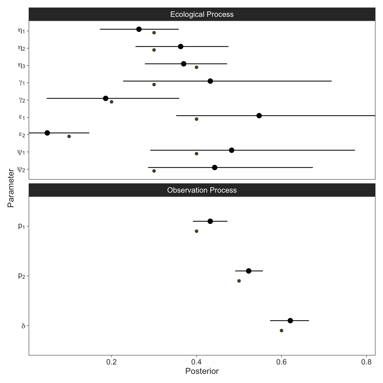
Let’s also check how many of our ecological ecological states were correctly recovered. Since only state 3 (snakes present and breeding) can be directly observed with certainty, we’ll only check the ecological states for those times where no breeding was observed.
Code
# A tibble: 1 × 1
  prop_true
      <dbl>
1 0.643ChatGPT tells me that to get the steady state distribution from a TPM, you perform the eigendecomposition of the TPM and the eigenvector corresponding to the eigenvalue of 1 is the steady state distribution. Stan does have eigendecomposition, so I’m sure there’s a way to parameterise the initial states nicely, but it gets more complicated with time- and/or individual-varying parameters.
Example 3: Disease-structured mark-recapture with state misclassification
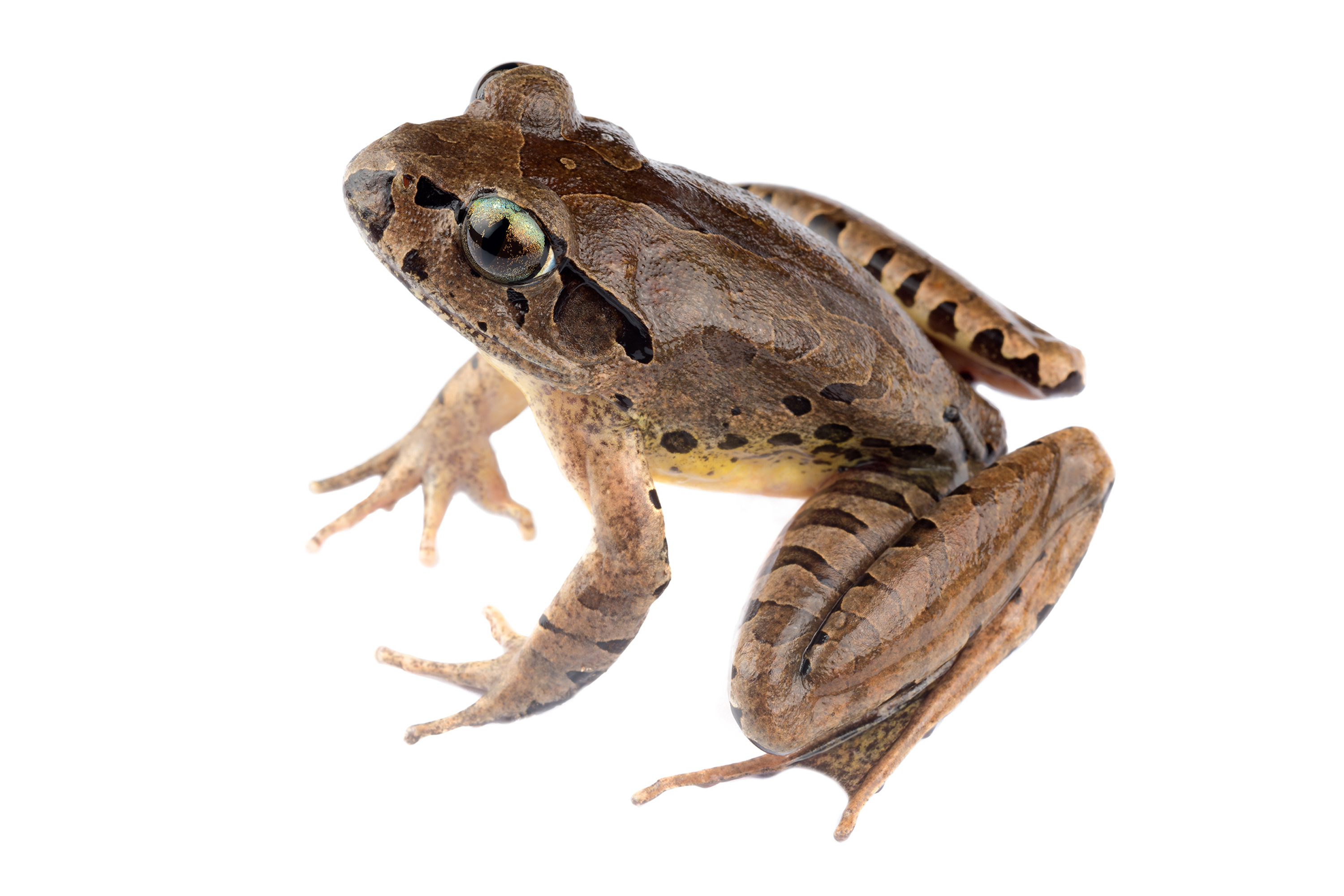
The main reason I dove so deep into HMMs is because during my PhD I ran into a problem with my mark-recapture study on Fleay’s barred frogs (Mixophyes fleayi). For two years I conducted mark-recapture surveys along Gondwana rainforest streams in northern New South Wales, Australia, swabbing every frog I found to test for the presence of the pathogenic amphibian chytrid fungus (Batrachochytrium dendrobatidis, Bd) (Scheele et al. 2019) to hopefully infer something about (1) the effect of Bd on frog mortality rates and (2) the infection dynamics.
The ecological TRM of such a disease-structured multistate model is pretty straightforward, with three possible states: (1) alive and uninfected, (2) alive and infected, and (3) dead, which is an absorbing state:
\[ Q = \begin{bmatrix} -(\psi_1 + \phi_1) & \psi_1 & \phi_1 \\ \psi_2 & -(\psi_2 + \phi_2) & \phi_2 \\ 0 & 0 & 0 \end{bmatrix} \tag{10}\]
Here, \(\phi_{1:2}\) are the mortality hazard rates of uninfected and infected frogs, respectively, and \(\psi_{1:2}\) are the rates of gaining and clearing infections, respectively.
Nothing is certain
While I was running qPCRs in the lab on some swabs collected during high frequency surveys (1 week intervals) with large numbers of recaptures, I noticed some frogs were apparently frequently clearing and re-gaining infections. For instance, a frog captured on 5 successive weeks may have looked something like this: \(\left[ 2, 2, 1, 2, 1 \right]\), implying the infection was lost twice and gained once across 4 weeks. This seemed unlikely, and it struck me as more probable that I was simply getting false negatives. At the same time, I couldn’t rule out false positives, either, given that contamination is always a risk. The best way to account for this uncertainty is to model it.
I realised that if you conduct robust design sampling and collect a swab with each capture, you could essentially model the swabbing process like an occupancy model within a mark-recapture model. That is, imagine surveying frogs \(i \in 1:I\) during \(j \in 1:J\) primary occasions (say every 2 months). During each primary occasion, you conduct multiple secondary surveys \(k \in 1:K_j\) within a short amount of time where you’re willing to assume the population is closed, that is, no animals dying, coming in, changing their infection state, etc. Every time you capture a frog, including those captured multiple times within a primary, you collect a swab. There are 3 possible observed states (\(o\)) per secondary: (1) frog captured with swab Bd–, (2) frog captured with swab Bd+, and (3) frog not captured. The TPM of this observation process for repeat secondaries with false negatives and false positives is as follows, with ecological states in the rows and observed states in the columns:
\[ P_o = \begin{bmatrix} p_1 \cdot ( 1 - \lambda_1) & p_2 \cdot \lambda_1 & 1 - p_1 \\ p_2 \cdot (1 - \delta_1) & p_2 \cdot \delta_1 & 1 - p_2 \\ 0 & 0 & 1 \end{bmatrix} \tag{11}\] Where \(p_{1:2}\) are the detection probabilities of uninfected and infected frogs, respectively, \(\lambda_1\) is the probability of getting a Bd+ swab from an uninfected frog (false positive), and \(\delta_2\) is the probability of detecting Bd on a swab from an infected frog (where \(1 - \delta_1\) is the false negative probability). The Bd detection parameters \(\delta_1\) and \(\lambda_1\) are identified if at least some frogs are recaptured multiple times within a primary occasion.
Double-decking the HMM
This is already a lot, but it’s really no different from Example 2: a continuous time ecological process, simpler this time because the dead state is absorbing, and a discrete time observation process, albeit with an extra false positive parameter. However, the reality of the data was slightly more complex. It is conventional to run qPCR several times per swab to accurately quantify the DNA load present in a sample. But this is analogous to the swabbing process described above. Presumably, it’s possible to get false negatives and false positives in the qPCR diagnostic process as well. There are thus three diagnostic states (\(y\), data): (1) qPCR replicate Bd–, (2) qPCR replicate Bd+, or (3) no qPCR performed, because no frog was captured and thus no swab was collected. Typically, people will just average their measured DNA loads across runs and apply an inclusion criterion, such as that samples are considered infected when 2/3 qPCR replicates return Bd DNA. But we can do better by just modeling it. Here’s the TPM of the diagnostic process, with latent observed states in the rows and diagnostic states in the columns:
\[ P_y = \begin{bmatrix} 1 - \lambda_2 & \lambda_2 & 0 \\ 1 - \delta_2 & \delta_2 & 0 \\ 0 & 0 & 1 \end{bmatrix} \tag{12}\] where \(\lambda_2\) is another false positive parameter and \(\delta_2\) is the detection probability in the qPCR process.
Always try to use all of the data
Another element of this model involved incorporating infection intensity into the model. qPCR doesn’t just tell you whether a sample is infected, but it tells you how many DNA copies are present in the sample. So with infection intensities \(x\) from multiple qPCR runs \(l \in 1:L\) collected from multiple samples (\(n\)), we can actually estimate the latent infection intensity on the individual \(m\) and samples:
\[ \begin{aligned} m_{i,j} &\sim \mathrm{Lognormal} \left( \mu, \sigma_1 \right) \\ n_{i,j,k} &\sim \mathrm{Lognormal} \left( m_{i,j}, \sigma_2 \right) \\ x_{i,j,k,l} &\sim \mathrm{Lognormal} \left( n_{i,j,k}, \sigma_3 \right) \end{aligned} \tag{13}\] where lognormals are used to ensure the infection intensities are positive, \(\mu\) is the log population average and \(\sigma_{1:3}\) are the population standard deviation and the errors of the swabbing and qPCR processes, respectively. One could of course model the individual infection intensities \(m_{ij}\) more flexibly as individual-level time series, but my data was too sparse and probably way too noisy. We can now incorporate the infection intensities to the ecological and observation models by modeling \(\phi_2\), the mortality rates of infected frogs, and \(\delta_{1:2}\), the Bd detection probabilities, as functions of the relevant infection intensities, for example like this:
\[ \begin{aligned} {\phi_2}_{[i, j]} &= \exp \left( \log {\phi_2}_\alpha + {\phi_2}_\beta \cdot m_{i,j} \right) \\ {\delta_1}_{[i,j]} &= 1 - (1 - r_1)^{m_{i,j}} \\ {\delta_2}_{[i,j,k]} &= 1 - (1 - r_2)^{n_{i,j,k}} \end{aligned} \tag{14}\] Here, the first equation is a simple GLM of the mortality hazard rate as a function of time-varying individual infection intensity, and the Bd detection probabilities are modeled as a function of \(r_{1:2}\), or the probabilities of detecting one log gene copy of DNA on a swab or qPCR replicate.
Dr. Andy Royle and myself published this model in Methods in Ecology and Evolution where we initially implemented the model in NIMBLE (Hollanders and Royle 2022). But of course, I was keen to try to marginalise out the latent ecological and observed states to fit this model in Stan (note that the ecological states are completely unobserved, as there’s no way of knowing whether an infected qPCR run actually came from an infected sample or frog!).
Simulation
Below I simulate some data where the rates of gaining and clearing infection are also affected by temperature (negative and positive, respectively), which seems to be the case for the frog-Bd system.4 To account for the varying infection dynamics in the state probabilities at first capture, I’ll use the steady state distribution for each primary which is computed using the infection dynamics probabilities, given by \({\psi_p}_{[1:2]} = 1 - \exp(-\psi_{1:2})\). Then, the expected probability of being infected at first capture in each primary is \(\eta = \frac{{\psi_p}_{[1]}}{{\psi_p}_{[1]} + {\psi_p}_{[2]}}\).
Code
# metadata
I <- 100
J <- 8
K_max <- 3
K <- rep(K_max, J)
L <- 3
tau <- rlnorm(J - 1, log(1), 0.5)             # unequal primary occasion intervals
temp <- rnorm(J - 1) |> sort(decreasing = T)  # it's getting colder

# parameters
phi_a <- c(0.1, 0.1)       # mortality rates of uninfected/infected frogs (intercepts)
phi_b <- 0.3               # effect of one log Bd gene copy on mortality
psi_a <- c(0.7, 0.4)       # rates of gaining/clearing infections (intercepts)
psi_b <- c(-0.4, 0.3)      # effect of temperature on rates of gaining/clearing infections
p_a <- c(0.7, 0.6)         # detection probabilities of uninfected/infected frogs
r <- c(0.4, 0.6)           # pathogen detection probabilities (per log Bd gene copy)
lambda <- c(0.05, 0.10)    # sampling/diagnostic false positive probabilities
mu <- 1.0                  # population log average infection intensity
sigma <- c(0.3, 0.2, 0.1)  # population and sampling/diagnostic SDs

# parameter containers
phi <- matrix(phi_a, 2, J - 1)
psi <- exp(matrix(log(psi_a), 2, J - 1) + psi_b %*% t(temp))
psi_p <- 1 - exp(-psi)
eta <- psi_p[1, ] / colSums(psi_p)
p <- array(p_a, c(2, J, K_max))
delta1 <- numeric(J)
delta2 <- matrix(NA, J, K_max)
m <- matrix(NA, I, J)
n <- array(NA, c(I, J, K_max))

# TPM containers
Q <- P_z <- array(NA, c(3, 3, J - 1))
P_o <- array(NA, c(3, 3, J, K_max))
P_y <- array(NA, c(3, 3, J, K_max))

# primary occasions of first capture
f <- sort(sample(1:(J - 1), I, replace = T))

# containers
z <- matrix(NA, I, J)
o <- array(NA, c(I, J, K_max))
y <- x <- array(NA, c(I, J, K_max, L))

# simulate
for (i in 1:I) {

  # fix detection probabilities in first secondary of first primary to ensure capture
  p[, f[i], 1] <- 1

  for (j in f[i]:J) {

    # infection intensities and pathogen detection probabilities
    m[i, j] <- rlnorm(1, mu, sigma[1])
    delta1[j] <- 1 - (1 - r[1])^m[i, j]
    n[i, j, 1:K[j]] <- rlnorm(K[j], log(m[i, j]), sigma[2])
    delta2[j, 1:K[j]] <- 1 - (1 - r[2])^n[i, j, 1:K[j]]

    # observation and diagnostic TPMs
    for (k in 1:K[j]) {
      P_o[, , j, k] <- matrix(c(p[1, j, k] * (1 - lambda[1]), p[1, j, k] * lambda[1], 1 - p[1, j, k],
                                p[2, j, k] * (1 - delta1[j]), p[2, j, k] * delta1[j], 1 - p[2, j, k],
                                0, 0, 1),
                              3, byrow = T)
      P_y[, , j, k] <- matrix(c(1 - lambda[2], lambda[2], 0,
                                1 - delta2[j, k], delta2[j, k], 0,
                                0, 0, 1),
                              3, byrow = T)
    }
  }

  # mortality rates and ecological TRM/TPMs
  for (j in f[i]:(J - 1)) {
    phi[2, j] <- exp(log(phi_a[2]) + phi_b * m[i, j])
    Q[, , j] <- matrix(c(-(psi[1, j] + phi[1, j]), psi[1, j], phi[1, j],
                         psi[2, j], -(psi[2, j] + phi[2, j]), phi[2, j],
                         0, 0, 0),
                       3, byrow = T)
    P_z[, , j] <- expm(Q[, , j] * tau[j])
  }

  # ecological process
  z[i, f[i]] <- rcat(1, c(1 - eta[f[i]], eta[f[i]]))
  for (j in (f[i] + 1):J) {
    z[i, j] <- rcat(1, P_z[z[i, j - 1], , j - 1])
  }

  # observation and diagnostic process
  for (j in f[i]:J) {
    for (k in 1:K[j]) {
      o[i, j, k] <- rcat(1, P_o[z[i, j], , j, k])
      y[i, j, k, ] <- rcat(L, P_y[o[i, j, k], , j, k])

      # diagnostic run infection intensity
      for (l in 1:L) {
        if (y[i, j, k, l] == 2) {
          x[i, j, k, l] <- rlnorm(1, log(n[i, j, k]), sigma[3])
        }
      }
    }
  }
}
Stan implementation
This model took me a lot of time to get going in Stan, but I got there in the end. I won’t go into detail about explaining everything, but I’ll mention a few key things here:
- We only need to account for the pathogen detection components between an individual’s first and last primary of capture, because no samples are collected when an individual isn’t captured. This means \(P_o\) and \(P_y\) can be constructed as \(2 \cdot 2\) matrices corresponding to the two alive states. Since this model doesn’t include any variation on detection, I created a vector
lp_not_detectedwhich holds the marginal log probabilities of not being detected for all three states, which is just \(\log\left([1 - p_1, 1 - p_2, 1\right]^\intercal)\). - Robust design sampling means we can actually model the detection probabilities of the first primary. We do have to fix the first secondary that the individual was caught to 1, but are free to estimate the remaining detection probabilities.
- The marginal log probabilities
Omegaare initialised with the observation and diagnostic TPMs for each secondary. This involves a sort of intermediate forward algorithm, where I (log) matrix multiply the observation TPM with the marginal log probabilities of the diagnostic outcomes (summing the log probabilities of each diagnostic run for each state, for which I created arow_sums()function). - The inclusion of false positives means the observation and diagnostic processes are examples of finite mixtures that may have multimodality in certain model constructions (Royle and Link 2006). Here, the true pathogen detection probabilities \(\delta\) are modeled as a function of infection intensity, which may be enough to avoid the multimodality. Just to be sure, however, I’ve constrained \(\lambda_{1:2}\) to be less than \(r_{1:2}\) in the program and further supplied \(\mathrm{Beta} (1, 10)\) priors for \(\lambda\).
- The individual infection intensities
m[i, j]are parameterised as centered lognormal and the sample infection intensitiesn[i, j, k]as non-centered lognormal, as this seemed to give the best HMC performance.
Code
functions {
  // normalise a vector of log probabilities
  vector normalise_log(vector A) {
    return A - log_sum_exp(A);
  }

  /**
   * Return the natural logarithm of the product of the element-wise
   * exponentiation of the specified matrices
   *
   * @param A  First matrix or (row_)vector
   * @param B  Second matrix or (row_)vector
   *
   * @return   log(exp(A) * exp(B))
   */
  matrix log_prod_exp(matrix A, matrix B) {
    int I = rows(A);
    int J = cols(A);
    int K = cols(B);
    matrix[J, I] A_tr = A';
    matrix[I, K] C;
    for (k in 1:K) {
      for (i in 1:I) {
        C[i, k] = log_sum_exp(A_tr[:, i] + B[:, k]);
      }
    }
    return C;
  }
  vector log_prod_exp(matrix A, vector B) {
    int I = rows(A);
    int J = cols(A);
    matrix[J, I] A_tr = A';
    vector[I] C;
    for (i in 1:I) {
      C[i] = log_sum_exp(A_tr[:, i] + B);
    }
    return C;
  }
  row_vector log_prod_exp(row_vector A, matrix B) {
    int K = cols(B);
    vector[size(A)] A_tr = A';
    row_vector[K] C;
    for (k in 1:K) {
      C[k] = log_sum_exp(A_tr + B[:, k]);
    }
    return C;
  }
  real log_prod_exp(row_vector A, vector B) {
    return log_sum_exp(A' + B);
  }

  /**
   * Row- or column sums of a matrix
   *
   * @param A  Matrix
   *
   * @return   (Row-)vector with the sums of each row or column
   */
  vector row_sums(matrix A) {
    int I = rows(A);
    vector[I] B;
    for (i in 1:I) {
      B[i] = sum(A[i]);
    }
    return B;
  }
  row_vector col_sums(matrix A) {
    int J = cols(A);
    row_vector[J] B;
    for (j in 1:J) {
      B[j] = sum(A[:, j]);
    }
    return B;
  }
}

data {
  int<lower=0> I, J, K_max, L, S;
  array[J] int<lower=1, upper=K_max> K;
  array[I] int<lower=1, upper=J> f;
  array[I] int<lower=f, upper=J> l;
  array[I] int<lower=1, upper=K_max> f_k;
  vector<lower=0>[J - 1] tau;
  row_vector[J - 1] temp;
  array[I, J, K_max, L] int<lower=1, upper=3> y;
  array[S] int<lower=1> ind, prim, sec;
  vector[S] x;
}

transformed data {
  array[I, J, K_max] int q;  // detected during secondary
  int M = 0, N = 0;  // number of parameters for individual and sample loads
  for (i in 1:I) {
    for (j in f[i]:J) {
      M += 1;
      for (k in 1:K[j]) {
        q[i, j, k] = min(y[i, j, k]) < 3;
        N += 1;
      }
    }
  }
}

parameters {
  vector<lower=0>[2] phi_a, psi_a;
  real phi_b;
  vector[2] psi_b;
  vector<lower=0, upper=1>[2] p_a, r;
  vector<lower=0, upper=r>[2] lambda;
  real mu;
  vector<lower=0>[3] sigma;
  vector[M] log_m;
  vector[N] log_n_z;
}

model {
  // priors
  target += exponential_lupdf(phi_a | 1);
  target += std_normal_lupdf(phi_b);
  target += exponential_lupdf(psi_a | 1);
  target += std_normal_lupdf(psi_b);
  target += beta_lupdf(p_a | 1, 1);
  target += beta_lupdf(r | 1, 1);
  target += beta_lupdf(lambda | 1, 10);
  target += normal_lupdf(mu | 0, 1);
  target += exponential_lupdf(sigma | 1);
  target += normal_lupdf(log_m | mu, sigma[1]);
  target += std_normal_lupdf(log_n_z);

  // fill in individual and sample infection containers
  matrix[I, J] m;
  array[I] matrix[J, K_max] n;
  int m_idx = 1, n_idx = 1;
  for (i in 1:I) {
    for (j in f[i]:J) {
      m[i, j] = log_m[m_idx];
      m_idx += 1;
      if (j <= l[i]) {
        for (k in 1:K[j]) {
          n[i][j, k] = m[i, j] + log_n_z[n_idx] * sigma[2];
          n_idx += 1;
        }
      }
    }
  }

  // likelihood of diagnostic infection intensities
  for (s in 1:S) {
    target += lognormal_lupdf(x[s] | n[ind[s]][prim[s], sec[s]], sigma[3]);
  }

  // exponentiate log infection intensities
  m = exp(m);
  n = exp(n);

  // ecological rates and initial state log probabilities
  matrix[2, J - 1] phi = rep_matrix(phi_a, J - 1);
  matrix[2, J - 1] psi = exp(rep_matrix(log(psi_a), J - 1) + psi_b * temp);
  matrix[2, J - 1] psi_p = 1 - exp(-psi);
  row_vector[J - 1] eta = psi_p[1] ./ col_sums(psi_p);
  row_vector[J - 1] log_eta = log(eta), log1m_eta = log1m(eta);

  // containers
  vector[3] lp_not_detected = append_row(log1m(p_a), 0);  // undetected vector
  tuple(row_vector[J], matrix[J, K_max]) delta;
  array[J - 1] matrix[3, 3] Q, P_z;
  matrix[2, 2] P_o, P_y;
  matrix[3, J] Omega;

  // for each individual
  for (i in 1:I) {

    // overwite mortality rates of infected
    phi[2][f[i]:(J - 1)] = exp(log(phi_a[2]) + phi_b * m[i, f[i]:(J - 1)]);

    // ecological TRMs and (log) TPMs (Stan doesn't like the log of all 0s)
    for (j in f[i]:(J - 1)) {
      Q[j] = [[ -(psi[1, j] + phi[1, j]), psi[1, j], phi[1, j] ],
              [ psi[2, j], -(psi[2, j] + phi[2, j]), phi[2, j] ],
              zeros_row_vector(3) ];
      P_z[j][1:2] = log(matrix_exp(Q[j] * tau[j])[1:2]);
      P_z[j][3] = [ negative_infinity(), negative_infinity(), 0 ];
    }

    // pathogen detection only needed for observed primaries
    delta.1[f[i]:l[i]] = 1 - pow(1 - r[1], m[i, f[i]:l[i]]);
    delta.2[f[i]:l[i]] = 1 - pow(1 - r[2], n[i][f[i]:l[i]]);

    // initialise log probabilities
    Omega = rep_matrix(0, 3, J);

    // for each primary between first and last capture
    for (j in f[i]:l[i]) {
      for (k in 1:K[j]) {

        // fix detection probablity to 1 at secondary of first capture
        vector[2] p = (j == f[i] && k == f_k[i]) ? ones_vector(2) : p_a;

        // observation and diagnostic (log) TPMs
        P_o = [[ p[1] * (1 - lambda[1]), p[1] * lambda[1] ],
               [ p[2] * (1 - delta.1[j]), p[2] * delta.1[j] ]];
        P_y = [[ 1 - lambda[2], lambda[2] ],
               [ 1 - delta.2[j, k], delta.2[j, k] ]];
        P_o = log(P_o);
        P_y = log(P_y);

        // increment observation and diagnostic process if detected
        if (q[i, j, k]) {
          Omega[1:2, j] += log_prod_exp(P_o, row_sums(P_y[:, y[i, j, k]]));
        } else {
          Omega[1:2, j] += lp_not_detected[1:2];
        }
      }
    }

    // increment ecological process up to last capture
    Omega[1:2, f[i]] += [ log1m_eta[f[i]], log_eta[f[i]] ]';
    for (j in (f[i] + 1):l[i]) {
      Omega[1:2, j] += log_prod_exp(P_z[j - 1][1:2, 1:2]', Omega[1:2, j - 1]);
    }
    Omega[3, l[i]] = negative_infinity();

    // increment ecological and observation process after last capture
    for (j in (l[i] + 1):J) {
      Omega[:, j] += log_prod_exp(P_z[j - 1]', Omega[:, j - 1]);
      for (k in 1:K[j]) {
        Omega[:, j] += lp_not_detected;
      }
    }

    // increment log density
    target += log_sum_exp(Omega[:, J]);
  }
}

generated quantities {
  vector[I] log_lik;
  array[I, J] int z;
  {
    matrix[I, J] m;
    array[I] matrix[J, K_max] n;
    int m_idx = 0, n_idx = 0;
    for (i in 1:I) {
      for (j in f[i]:J) {
        m_idx += 1;
        m[i, j] = log_m[m_idx];
        if (j <= l[i]) {
          for (k in 1:K[j]) {
            n_idx += 1;
            n[i][j, k] = m[i, j] + log_n_z[n_idx] * sigma[2];
          }
        }
      }
    }
    m = exp(m);
    n = exp(n);
    matrix[2, J - 1] psi = exp(rep_matrix(log(psi_a), J - 1) + psi_b * temp);
    matrix[2, J - 1] psi_p = 1 - exp(-psi);
    row_vector[J - 1] eta = psi_p[1] ./ col_sums(psi_p);
    row_vector[J - 1] log_eta = log(eta), log1m_eta = log1m(eta);
    vector[3] lp_not_detected = append_row(log1m(p_a), 0);
    tuple(row_vector[J], matrix[J, K_max]) delta;
    array[J - 1] matrix[3, 3] Q, P_z;
    matrix[2, 2] P_o, P_y;
    matrix[3, J] Omega;
    for (i in 1:I) {
      matrix[2, J - 1] phi;
      phi[1] = rep_row_vector(phi_a[1], J - 1);
      phi[2][f[i]:(J - 1)] = exp(log(phi_a[2]) + phi_b * m[i, f[i]:(J - 1)]);
      for (j in f[i]:(J - 1)) {
        Q[j] = [[ -(psi[1, j] + phi[1, j]), psi[1, j], phi[1, j] ],
                [ psi[2, j], -(psi[2, j] + phi[2, j]), phi[2, j] ],
                zeros_row_vector(3) ];
        P_z[j][1:2] = log(matrix_exp(Q[j] * tau[j])[1:2]);
        P_z[j][3] = [ negative_infinity(), negative_infinity(), 0 ];
      }
      delta.1[f[i]:l[i]] = 1 - pow(1 - r[1], m[i, f[i]:l[i]]);
      delta.2[f[i]:l[i]] = 1 - pow(1 - r[2], n[i][f[i]:l[i]]);
      Omega = rep_matrix(0, 3, J);
      for (j in f[i]:l[i]) {
        for (k in 1:K[j]) {
          vector[2] p = (j == f[i] && k == f_k[i]) ? ones_vector(2) : p_a;
          P_o = [[ p[1] * (1 - lambda[1]), p[1] * lambda[1] ],
                 [ p[2] * (1 - delta.1[j]), p[2] * delta.1[j] ]];
          P_y = [[ 1 - lambda[2], lambda[2] ],
                 [ 1 - delta.2[j, k], delta.2[j, k] ]];
          P_o = log(P_o);
          P_y = log(P_y);

          // forward algorithm for log likelihood
          if (q[i, j, k]) {
            Omega[1:2, j] += log_prod_exp(P_o, row_sums(P_y[:, y[i, j, k]]));
          } else {
            Omega[1:2, j] += lp_not_detected[1:2];
          }
        }
      }
      Omega[1:2, f[i]] += [ log1m_eta[f[i]], log_eta[f[i]] ]';
      for (j in (f[i] + 1):l[i]) {
        Omega[1:2, j] += log_prod_exp(P_z[j - 1][1:2, 1:2]', Omega[1:2, j - 1]);
      }
      Omega[3, l[i]] = negative_infinity();
      for (j in (l[i] + 1):J) {
        Omega[:, j] += log_prod_exp(P_z[j - 1]', Omega[:, j - 1]);
        for (k in 1:K[j]) {
          Omega[:, j] += lp_not_detected;
        }
      }
      log_lik[i] = log_sum_exp(Omega[:, J]);

      // backward algorithm for ecological states
      z[i, J] = categorical_rng(exp(normalise_log(Omega[:, J])));
      for (j in (f[i]) + 1:J) {
        int jj = J + f[i] - j;
        z[i, jj] = categorical_rng(exp(normalise_log(Omega[:, jj]
                                                     + P_z[jj][:, z[i, jj + 1]])));
      }
    }
  }
}
Next I convert the qPCR infection intensities to long format, prepare the data for Stan, and fit the model.
Code
# convert diagnostic infection intensities to long format
x_long <- reshape2::melt(x, value.name = "x", varnames = c("i", "j", "k", "l")) |>
  as_tibble() |>
  drop_na()

# data for Stan
f_k <- rep(1, I)  # simulated to be first captured in first secondary
l <- apply(y, 1:2, min, na.rm = T) |> apply(1, \(y) max(which(y < 3)))
multievent_data <- list(I = I, J = J, K_max = K_max, L = L, S = nrow(x_long),
                        K = K, f = f, l = l, f_k = f_k, tau = tau, temp = temp,
                        y = ifelse(is.na(y), 3, y),
                        ind = x_long$i, prim = x_long$j, sec = x_long$k,
                        x = x_long$x)


# run HMC
fit_multievent <- multievent$sample(data = multievent_data, refresh = 0, chains = n_chains,
                                    iter_warmup = n_iter, iter_sampling = n_iter)
Running MCMC with 8 parallel chains...Chain 1 finished in 375.4 seconds.
Chain 4 finished in 421.9 seconds.
Chain 6 finished in 422.6 seconds.
Chain 2 finished in 475.8 seconds.
Chain 3 finished in 502.1 seconds.
Chain 7 finished in 527.8 seconds.
Chain 8 finished in 586.8 seconds.
Chain 5 finished in 661.5 seconds.
All 8 chains finished successfully.
Mean chain execution time: 496.7 seconds.
Total execution time: 661.8 seconds.Results
We’ll visually check the parameter estimates with the simulation input and see that it was recovered well. For what it’s worth, in the paper we showed that the infection dynamics get overestimated significantly (5-fold in our application) when not accounting for state misclassification.
Code
fit_multievent |>
  gather_rvars(phi_a[i], phi_b, psi_a[i], psi_b[i], p_a[i], r[i], lambda[i], mu, sigma[i]) |>
  mutate(truth = c(phi_a, phi_b, psi_a, psi_b, p_a, r, lambda, mu, sigma),
         parameter = str_extract(.variable, "^[^_]+") |>
           fct_inorder(),
         process = case_when(str_detect(.variable, "phi|psi") ~ "Ecological Process",
                             str_detect(.variable, "p_a|r|lambda") ~ "Observation Process",
                             .default = "Infection Intensities") |>
           fct_inorder(),
         variable = case_when(str_detect(.variable, "_a") ~ str_c(parameter, "[", i, "[alpha]]"),
                              .variable == "phi_b" ~ "phi[beta]",
                              .variable == "psi_b" ~ str_c(parameter, "[", i, "[beta]]"),
                              .variable %in% c("r", "lambda", "sigma") ~ str_c(parameter, "[", i, "]"),
                              .default = .variable) |>
           fct_reorder(as.numeric(parameter))) |>
  ggplot(aes(xdist = .value, y = fct_rev(variable))) +
  facet_wrap(~ process, ncol = 1, scales = "free_y") +
  geom_vline(xintercept = 0, linetype = "dashed", colour = "#333333") +
  stat_pointinterval(point_interval = median_qi, .width = 0.9, linewidth = 0.5, position = position_nudge(y = 0.1)) +
  geom_point(aes(truth), colour = green, position = position_nudge(y = -0.1)) +
  scale_x_continuous(breaks = seq(-1, 1, 0.5), expand = c(0, 0)) +
  scale_y_discrete(labels = ggplot2:::parse_safe) +
  labs(x = "Posterior", y = "Parameter")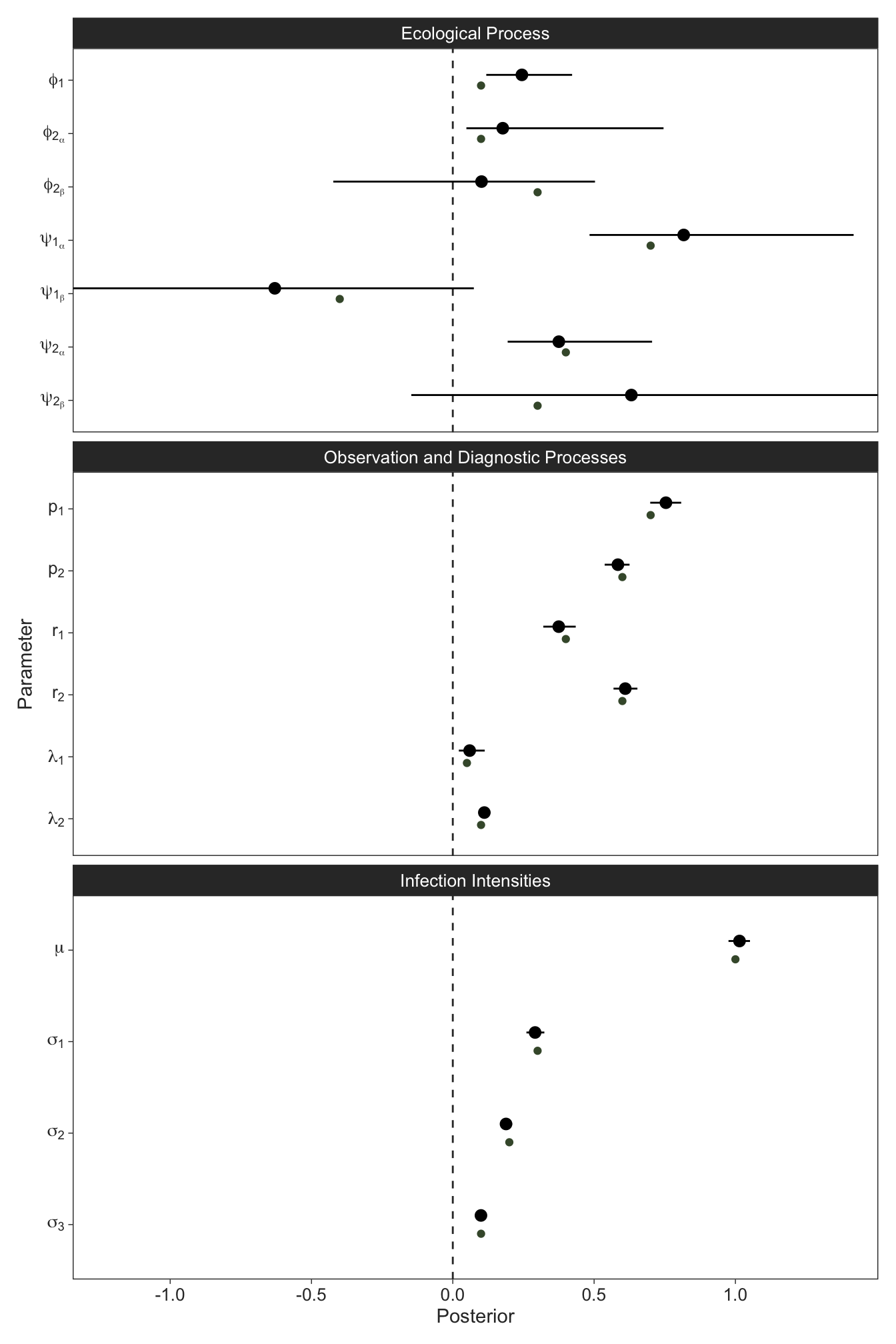
Again, we might check to see how well we recovered our latent ecological states, which were completely unobservable from the data. This worked pretty well!
Code
# A tibble: 1 × 1
  prop_true
      <dbl>
1     0.908
One of the main reasons to account for imperfect pathogen detection is to get more realistic estimates of infection prevalence in the population. We can use the full posterior distribution of the latent ecological states from the backward algorithm to estimate the infection prevalence per primary occasion, which here was simulated to be increasing due to dropping temperatures going into austral winter plotted for some fictional dates to show the unequal primary occasion intervals.
Code
# dates
start <- ymd("2020-12-01")
time_unit <- 21
dates <- seq.Date(start, start + days(1 + round(sum(tau) * time_unit)), by = 1)
prim <- dates[c(1, sapply(1:(J - 1), \(t) round(sum(tau[1:t] * time_unit))))]

# plot
library(posterior)
out |>
  left_join(tibble(j = 1:J,
                   prim = prim),
            by = "j") |>
  summarise(prev = rvar_sum(z == 2) / rvar_sum(z < 3),
            truth = sum(truth == 2) / sum(truth < 3),
            .by = prim) |>
  ggplot(aes(prim, truth, ydist = prev)) +
  stat_pointinterval(point_interval = median_qi, .width = 0.9, linewidth = 0.5, position = position_nudge(x = 0.2)) +
  geom_point(colour = green, position = position_nudge(x = -2)) +
  scale_y_continuous(breaks = seq(0.2, 1, 0.2), limits = c(0, 1.001), expand = c(0, 0)) +
  labs(x = "Primary Occasion", y = "Infection Prevalence")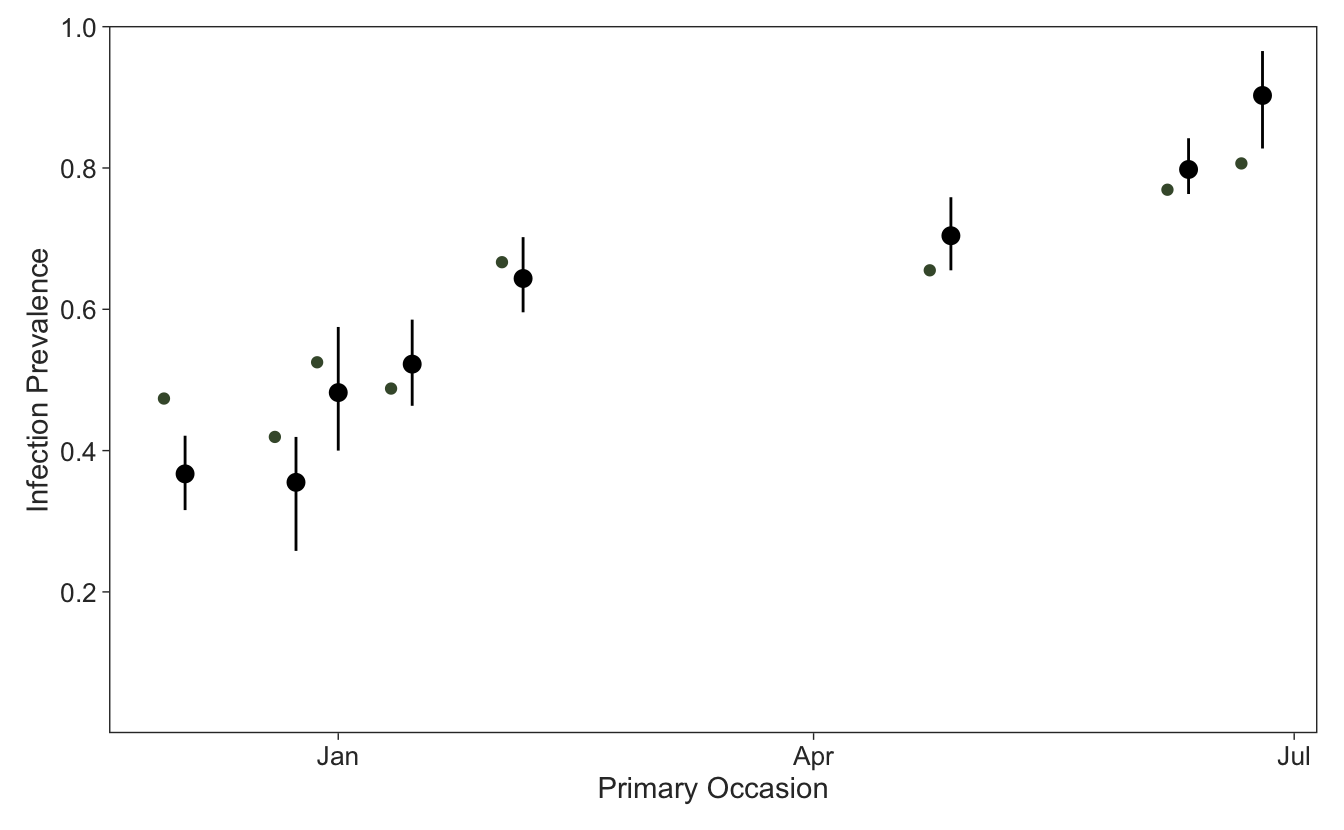
Thanks for reading if you made it this far. I hope this guide will be useful for ecologists (and others) wanting to transition to gradient-based sampling methods for complex ecological models. I’m sure I’ve some errors somewhere, so if someone finds any or has any questions, please don’t hesitate to reach out.
References
Footnotes
According to the Stan User’s Guide↩︎
Summing probabilities on the log scale requires exponentiating the log probabilities, summing them, and taking the logarithm once again.↩︎
There are some identifiability issues here, reflected in the posterior correlations that exist between the intercepts and slopes.↩︎